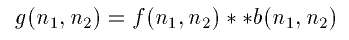
Inverse Filtering
If we know of or can create a good model of the blurring function
that corrupted an image, the quickest and easiest way to restore that is
by inverse filtering. Unfortunately, since the inverse filter is a form
of high pass filer, inverse filtering responds very badly to any noise
that is present in the image because noise tends to be high frequency.
In this section, we explore two methods of inverse filtering - a
thresholding method and an iterative method.
Method 1: Thresholding
Theory
We can model a blurred image by

In the ideal case, we would just invert all the elements of B to get a high pass filter. However, notice that a lot of the elements in B have values either at zero or very close to it. Inverting these elements would give us either infinities or some extremely high values. In order to avoid these values, we will need to set some sort of a threshold on the inverted element. So instead of making a full inverse out of B, we can an "almost" full inverse by
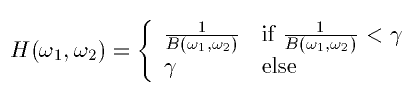
 , the closer H
is to the full inverse filter.
, the closer H
is to the full inverse filter.
Implementation and Results
Since Matlab does not deal well with infinity, we had to threshold
B before we took the inverse. So we did the following:
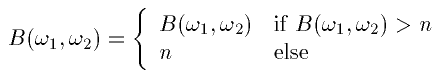
 and is set
arbitrarily close to zero for noiseless cases. The following images shows
our results for n=0.0001.
and is set
arbitrarily close to zero for noiseless cases. The following images shows
our results for n=0.0001.


We see that the image is almost exactly like the original. The MSE is 2.5847.
Because an inverse filter is a high pass filter, it does not perform
well in the presence of noise. There is a definite tradeoff between
de-blurring and de-noising. In the following image, the blurred image is
corrupted by AWGN with variance 10. n=0.2.

The MSE for the restored image is 1964.5. We can see that the sharpness of the edges improved but we also have a lot of noise specs in the image. We can get rid of more specs (thereby getting a smoother image) by increasing n. In general, the more noise we have in the image, the higher we set n. The higher the n, the less high pass the filter is, which means that it amplifies noise less. It also means, however, that the edges will not be as sharp as they could be.
Method 2: Iterative Procedure
Theory
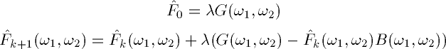
The idea behind the iterative procedure is to make some initial guess
of f based on g and to update that guess after every
iteration. The procedure is
where
 is an initial guess based on
g. If our
is an initial guess based on
g. If our  is a good guess,
eventually convolved with b will be
close to g. When that happens the second term in the
is a good guess,
eventually convolved with b will be
close to g. When that happens the second term in the
 equation will disappear and
and will
converge.
equation will disappear and
and will
converge.  is our convergence factor and it
lets us determine how fast and
converge.
is our convergence factor and it
lets us determine how fast and
converge.
If we take both of the above equations to the frequency domain, we
get
Solving for
 recursively, we get
So if
 goes to zero as k goes to
infinity, we would get the result as obtained by the inverse filter. In
general, this method will not give the exact same results as inverse
filtering, but can be less sensitive to noise in some cases.
goes to zero as k goes to
infinity, we would get the result as obtained by the inverse filter. In
general, this method will not give the exact same results as inverse
filtering, but can be less sensitive to noise in some cases.
Implementation and Results
The first thing we have to do is pick a
. must
satisfy the following
and thus will be a positive integer in the range of 0 to 1. The bigger
is, the faster
and will
converge. However, picking too large a may
also make and diverge instead of converge. Imagine that we're
walking along a path and the end of the path is a cliff. is the size of of the steps we take. We want
to go to the edge of the path as fast as possible without falling off.
Taking large steps will ensure that we will get there fast but we'd
probably first. Taking small will ensure that we get there without
falling off but it could take an infinite amount of time. So the
compromise would be to take big steps at the start and decrease our step
size as we get close to our destination.
The following is the noiseless image after 150 iterations.
starts off at 0.1 and decreases by 10%
every 25 iterations.
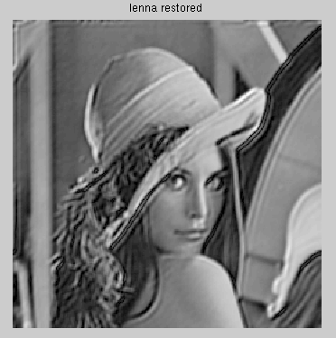
The MSE is 364.6897. The image is sharper than the blurred image although the MSE is high. But the image restored using the direct inverse filter is much better.
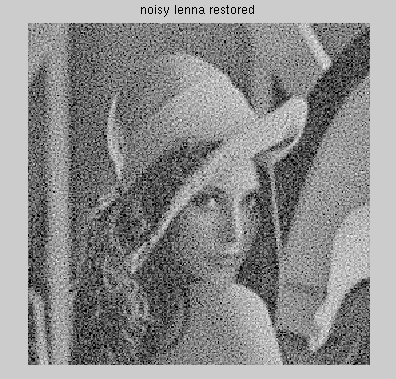
The following is the blurred image corrupted with AWGN with a
variance of 10. The number of iterations is 150.
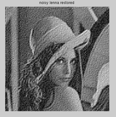
The MSE for the restored image is 1247.3. We see the same noise specs as we had seen with the inverse filter. But the image is in general better than the the noisy image restored using the inverse filtering method and has a lower MSE. So we can conclude that the direct inverse filtering method is better for a noiseless case and the iterative method is better when noise is present.
Follow the links below to view the matlab code:
inverse filter code
iterative method code