BLIND DECONVOLUTION
To this point, we have studied restoration techniques assuming that we knew the blurring function h . Actually, we have also assumed that we knew the image spectral density Suu and Spectral noise Snn as well. This section will focus on some techniques for estimating h based on our degraded image. For comparison, we will demonstrate how the MSE between our restored image and the original image changes depending on whether or not we know h, Suu, or Snn.
Two restoration filters will be the basis for our procedures. The first is the Wiener Filter, which exhibits the optimal tradeoff (in the MSE sense) between inverse filtering and noise smoothing. The second filter tries to restore the power spectrum of the degraded image, and is known as Power Spectrum Equalization [Lim].
We use as our degradation model the standard idea that our input image is blurred through convolution with a low pass LSI filter (h) and then Gaussian Noise is added to the result. Moreover, because Power Spectrum Equalization (PSE) works best assuming h is phaseless, so we generate our h to have zero phase. This is not too unrealistic because common degradations such as camera misfocus, uniform motion (linear phase), and atmospheric turbulence can all be modelled with zero phase filters. Note also that because we used a different filter for our degradation model than for Inverse Filtering and Wavelet Denoising, the MSEs of our restored images for this section should not be compared to those from the previous sections.
Let's begin by recalling the Wiener filter:
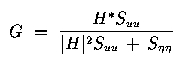
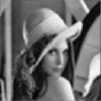
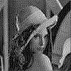
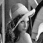
where H is the Fourier Transform of h, and Suu and Snn are defined as above. The following example shows lenna.256 degraded with our phaseless filter and AGN with variance 80. Suu is estimated as the magnitude squared of the Fourier Transform of the input image (lenna.256).
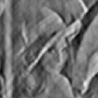
| Lenna after Blurring Plus Noise | Lenna restored using Wiener Filter |
 |
 |
| Mean Squared Error = 1.0660e+05 | Mean Squared Error = 123.2 |
The above images were generated using wien.m. Much of the blockiness is due to the compression we used on the gifs to store the images. This will be true for all the images in this section. The important things to note are the excellent reduction of MSE, and the improved definition in the boa of the restored image. In general, the blurriness of the degraded image has been removed.
Next we will examine the effectiveness of Power Spectrum Equalization. The equation is as follows:
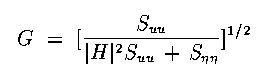
Note the similarity to Wiener Filtering, but we only use the magnitude of H. The following example demonstrates restoration using the same specs as for the Wiener Filter above.
| Lenna after Blurring Plus Noise | Lenna restored using PSE |
 |
 |
| Mean Squared Error = 1.0660e+05 | Mean Squared Error = 419.5 |
The above images were generated using pse.m. We have again removed a great deal of the blur, but our restoration is not as good as with Wiener Filtering. In general, Wiener filtering is the optimal restoration technique, and this should be remembered later on.
Next we will perform the same restoration using estimated spectral noise. For this we will assume that the noise is white and therefore has a flat (constant) spectral density. Experimentation showed us that overestimating the noise was better than underestimating the noise. This is due to the high pass characteristic of inverse filtering during restoration. When in doubt, suppress the inverse filter. The degraded images below where generated the same way as before, but Snn was estimated as 100.
| Lenna restored using Wiener Filtering | Lenna restored using PSE |
 |
 |
| Mean Squared Error = 252.6 | Mean Squared Error = 1.3932e+05 |
The above images were generated using wien2.m and pse2.m, respectively. Clearly, Power Spectrum Equalization is not very robust. A precise representation of the noise is required. This is because PSE does not use inverse filtering, so the noise estimation is doubly important. The code was checked thoroughly, and the only difference between this restoration and the one above was the estimation of Snn.
Our final preliminary investigation was to see what happens when we know h and Snn but not Suu. We estimated the image spectral density as the magnitude squared of the Fourier Transform of the degraded image (rather than of the original image, as before). The degradation was the same as before.
| Lenna restored using Wiener Filtering | Lenna restored using PSE |
 |
 |
| Mean Squared Error = 132.4 | Mean Squared Error = 371.9 |
The above images were generated using wien3.m and pse3.m, respectively. Again, we see that the Wiener filter has a lower MSE than the PSE filter. Also, for the Wiener Filter, our MSE isn't much worse than when we estimate Suu from the original image. For the PSE, our MSE has actually improved! We attribute this to the fact that our estimation of Suu isn't exact in either case. So generally, using the degraded image to estimate Suu won't hurt us with either restoration filter. The biggest unknown that hurts us so far is Snn for the PSE filter.
BLIND DECONVOLUTION
Many different methods were attempted to restore our image when we don't explicitly know h. Most of them had very little success. The reasons will be explained as we explain the general approach we used. The methods for estimating h are known as Blind Deconvolution because our inverse filtering (deconvolution) is being performed without knowledge of our blurring function. The methods we used were all homomorphic ideas.
In general, our degradation is modeled as a convolution plus noise. In the frequency domain, convolution becomes multiplication. If we ignore the additive noise, we can take the log of the multiplication and get addition. Thus, the log of the FT of our degraded image DI is equal to the log of the FT of the original image OI plus the log of the Transfer Function H. Now that we have addition, we can use statistical estimation to estimate H and thus solve for OI.
The problem with this method is that in practice we can't ignore the noise. Therefore, we need ways to estimate the log of the multiplication of OI and H plus the Noise Spectrum. The first approach we had success with came from the Jain text. It uses the following estimate for H.
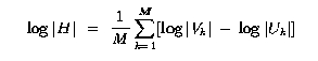
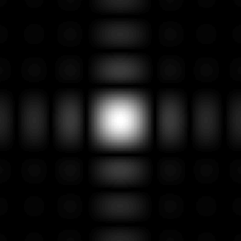
Uk and Vk are obtained by breaking the input image (u) and degraded image (v) into M smaller blocks and computing their Fourier Transforms. H is then used with Snn and Suu to compute the Wiener Filter. Notice that this method only computes Magnitude of H, so its best for phaseless LSI filters. This necessitated our filter design of a phaseless h. The following pictures show the Magnitude Plots of the actual and estimated transfer functions. Our image degration model is the same as always, and we calculated H using the above equation with M = 16. This broke down the images into 64x64 pixel blocks.
| Magnitude Plot of Blurring Filter | Magnitude Plot of Estimated Blurring Filter |
 |
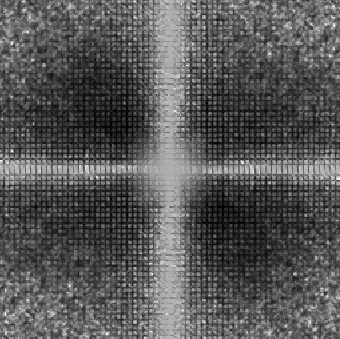 |
Note that we capture the form of the degradation filter, but we have a lot more noise. Surprisingly, our restoration MSE isn't too bad, depicted below. Both the above and below images were created using jain.m with noise variance 80. Also, since we are restoring using Wiener Filtering, we estimate Snn and Suu for restoration.
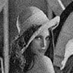
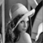
| Lenna after Blurring Plus Noise | Lenna restored using Jain Approach |
 |
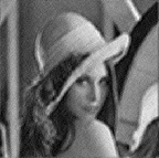 |
| Mean Squared Error = 1.0660e+05 | Mean Squared Error = 283.1 |
We see that our MSE has gone from 256 with unknown Snn to 283 with all three Wiener Filter componenents (h, Suu, * Snn). We can see that some of the blurring has been reduced in our restored image. Lines can be seen in the band around the hat and the boa is a bit clearer. However, even though our MSE isn't too bad, this is clearly the worst image restoration thus far with respect to visual aspects. Most of the restoration was magnitude restoration. But this was by far our greatest success at blind deconvolution.
Our second approach came from the Lim text. It was proposed by Stockham. The homomorphic idea of taking the log in the frequency domain is again present, as is the notion of breaking up the picture into M sub-blocks. The equation estimates the denominator of the PSE filter as follows:
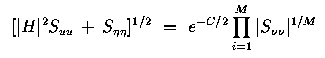
where C is Euler's constant (0.57221...). Note that H is never calculated directly. Instead, we use this estimation to choose our PSE filter and restore our image. Our attempt at restoration with this method is shown below. Again, variance is 80, but Suu and Snn are assumed known. Recall that if Snn is not explicitly known, then our PSE restoration fails.
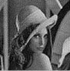
| Lenna after Blurring Plus Noise | Lenna restored using Stockham Approach |
 |
 |
| Mean Squared Error = 1.0656e+05 | Mean Squared Error = 7.4031e+07 |
The above images were generated using stockham.m. Clearly, our restoration has further degraded our image. This was seen earlier when we attempted PSE restoration without knowledge of Snn. In this case, we are trying to estimate the entire denominator, not just Snn. Our restoration suffers greatly.
We conclude that Power Spectrum Equalization is just a poor restoration choice in general. It fails for unknown Snn and for our attempt at unknown h. The lack of inverse filtering makes the denominator extremely important in restoration, so no estimation will be very robust. Supposedly, there are cases where PSE is preferable to Wiener Filtering [Castleman], but our models do not fit them.
There are direct methods for blind deconvolution as well, but we attempted only indirect methods, because they are less ad hoc. An example of a direct method for blind deconvolution is to model lines normal to a suspected edge in the degraded image as the integral of h, and use this measurement for deconvolution. Another indirect method we tried was to assume there was no additive noise in the system. Thus, if our average blurring function goes to zero over many images, we can estimate our original frequency information as the geometric mean of the degraded images. However, goemetric means are extremely vulnerable to noise, and many iterations were required for our approximations to hold. In general, we did not get good results for this method. You can view our code baran.m and try to improve it.
Further conclusions about Blind Deconvolution can be found in our Conclusions section.