The continuous back projection operator is defined by Eq. (5). Real data consists of a finite number of projections. For this project we have used the following approximate back projection formula:
In implementing the back projection algorithm, the following had to be considered:
Interpolation: The sum over all pixels, of all the rays that
passes through a particular pixel, as defined in Eq.
(8) has one minor problem: ![]() and f(x,y)
are in different coordinate systems. The expression for the s in
Eq. (8) takes care of this problem. It will,
however, require interpolation of
and f(x,y)
are in different coordinate systems. The expression for the s in
Eq. (8) takes care of this problem. It will,
however, require interpolation of ![]() to points between the
actual data points. According to reference [5] the best type
of interpolation is linear interpolation. Since we need to interpolate
over very long vectors and since the existing interpolation methods in
MATLAB execute slowly in this case, we implemented a linear
interpolation function in C. Our function takes advantage of the fact
that for any given value of
to points between the
actual data points. According to reference [5] the best type
of interpolation is linear interpolation. Since we need to interpolate
over very long vectors and since the existing interpolation methods in
MATLAB execute slowly in this case, we implemented a linear
interpolation function in C. Our function takes advantage of the fact
that for any given value of ![]() , the values of s for which we need
to approximate
, the values of s for which we need
to approximate ![]() are either monotonically increasing or
monotonically decreasing. This sped up the interpolation speed by
over an order of magnitude.
are either monotonically increasing or
monotonically decreasing. This sped up the interpolation speed by
over an order of magnitude.
Centering: Equation (8) assumes that the (x,y) coordinate system is centered in the middle of the image, while Matlab assumes it is centered in the upper left. We found that proper correction for centering is crucial to the success of the back projection algorithm. Even a small error causes severe artifacts.
Matrix formulation A straightforward implementation of the back
projection operation uses three nested loops, looping over each pixel
in the image, and for each pixel, through the different angles of
![]() . This leads to slow execution time in Matlab. Instead, we
employed a matrix formulation of the problem requiring only one loop,
over the different projections.
. This leads to slow execution time in Matlab. Instead, we
employed a matrix formulation of the problem requiring only one loop,
over the different projections.
As mentioned previously, the back projection operation produces a blurred version of the desired image. In the absence of noise, the desired image can be obtained by filtering the back projection with a ramp filter. Unfortunately, the high-pass nature of the ramp filter leads to amplification of high-frequency noise.
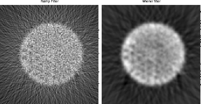
Figure 7: The left plot shows the reconstruction of the SPECT
phantom using the ramp filter. The right plot shows the
reconstructed image using a wiener filter.
As seen in Fig. 7 reconstruction using a ramp filter gives a very noisy image. We need to do some kind of low-pass filtering to reduce the noise. There will be a trade-off between a good ramp filter and noise suppression. The mean-squared optimal solution to this problem is a Wiener filter. Design of the Wiener filter requires knowledge about the statistics of the noise and the object. We modeled the noise as white Gaussian noise. We assumed the following covariance function for the image, inspired by reference [5]:
![]()
where ![]() and
and ![]() is the power spectral
density of the object. This expression states that the correlation
between two points decreases exponentially with distance, which seems
like a reasonable assumption. The Wiener filter in this case can be
expressed in the Fourier domain as:
is the power spectral
density of the object. This expression states that the correlation
between two points decreases exponentially with distance, which seems
like a reasonable assumption. The Wiener filter in this case can be
expressed in the Fourier domain as:
![]()
By investigating several cases we found that ![]() and SNR=60
produced good results. We tried various filter design techniques for
this filter, but obtained the best match to the ideal frequency
response as well as the best results with
and SNR=60
produced good results. We tried various filter design techniques for
this filter, but obtained the best match to the ideal frequency
response as well as the best results with ![]() optimal FIR
filters of length near 100. We originally expected such long filters
to cause edge effects, but since only the central part of
the image is of interest, no such effects are noticeable.
optimal FIR
filters of length near 100. We originally expected such long filters
to cause edge effects, but since only the central part of
the image is of interest, no such effects are noticeable.