 |
This simulation uses AspenPlus to model the plug flow reactor design created in the Matlab program plugr1, which simulates a plug flow reactor. Although a detailed description of building an Aspen model may be found elsewhere, this section briefly covers building a model of a reactor in Aspen.
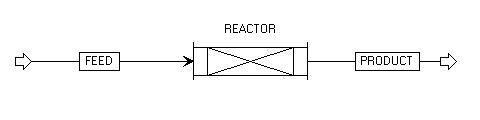
The only icon needed for this setup is a plug flow reactor icon (RPLUG). Your setup should look something like this after placing the icon with a feed stream and a product stream.
|
|
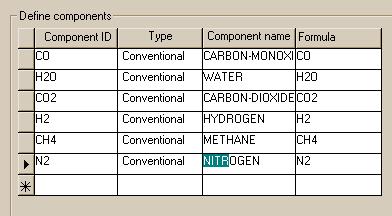
After the flowsheet is complete, it is time to specify the model. On the "Setup.Main" page, we let Aspen know that we would like to view the products as both mole flows and mole fractions. The "Components" window for this setup should look like this.
 |
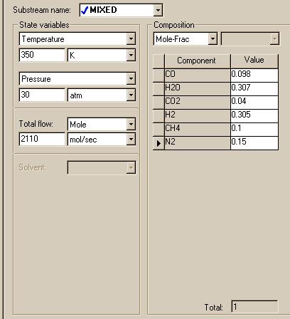
For the property set, choose ideal since the Matlab model of this reactor is based on ideal thermodynamics. When specifying the feed stream to the reactor, fill in your window such that it resembles this one. Keep in mind that these are the same conditions that may be found in the feed stream of the Matlab plug flow model.
 |
The next page of importance to appear is the "Rplug.Main" page. Note the section on this page entitled "Reactions." Since we are going to specify the reactions and the kinetics of the reactions that are going to occur in the reactor, we need to create a database on these reactions before we complete the "Rplug.Main" page. The first thing we have to do, though, is determine the kinetics of the system.
There are three reactions that are going to occur within the reactor.
Note that the second two equations are really the forward and reverse reactions of the same system. To model a reversible reaction in Aspen it must be treated as two reactions--forward and reverse.
Using kinetics, the following two rate equations may be written. Keep in mind that the first equation applies to the forward-only methane reaction, while the second equation incorporates both the forward and reverse reactions of the water-gas shift reaction.
r2 = DBED*A*e(-Ea2/(R*T))*yc*yw - DBED*A*e(-Ea2/(R*T))*yd*yh/keq(2)
Information about the variables may be found in the following table:
|
Variable |
Abbreviation |
Value |
Units |
|
Bed Density |
DBED |
1200 |
kg/m3 |
|
Pre-exponential Rate Constant |
km |
5.517e6 |
mol/kg/s/atm |
|
Activation Energy of Reaction 1 |
Ea1 |
1.849e8 |
J/mol |
|
Gas Constant |
R |
8.314 |
J/mol/K |
|
Pressure |
P |
30.0 |
atm |
|
Absorption Parameter |
Kh |
4.053 |
atm-1 |
|
Mole fraction of CH4 |
ym |
Varies |
Unitless |
|
Mole fraction of H2 |
yh |
Varies |
Unitless |
|
Mole fraction of CO |
yc |
Varies |
Unitless |
|
Mole fraction of H2O |
yw |
Varies |
Unitless |
|
Mole fraction of CO2 |
yd |
Varies |
Unitless |
|
Pre-exponential Constant |
A |
4.95e8 |
mol/kg/s |
|
Activation Energy of Reactions 2 |
Ea2 |
1.163e5 |
J/mol |
|
Equilibrium Constant1 |
keq(2) |
e-4.946 + 4897/T |
Unitless (T in K) |
1To determine the value of keq, the Matlab program kequil was used.
Consider the first reaction.
The form of the rate equation required by Aspen is a powerlaw equation, which has this form.
where Cm is the molar concentration of methane (P*ym/R/T). This relation is valid provided that the correct value of n is chosen and the gas behaves ideally.
In the Matlab example, the value of the mole fraction of hydrogen varies from 0.30 to about 0.38. This causes the value of (1 + Kh*P*yh) to vary from 36.5 to 46.2. Using an average of 41.4, we can compare both versions of the r1 equation to obtain
Therefore, to make these two equations equal to one another,
Once this has been determined, we need to make sure that the correct units are being employed. When using powerlaw equations in Aspen, the units used for the equation as a whole are based on the units used in the concentration variables. One of the choices Aspen has is molarity, which allows us to use kgmol/m3. To get k1 in the right units, we must do the following.
First, convert R (the Gas Constant) from J/mol/K to m3*atm/kgmol/K. We do this because of the units Aspen requires for kinetic data.:
        J             L*atm         m^3         mol            atm*m^3
8.314 ----- * 0.00987 ----- * 0.001 --- * 1000 ----- = 8.21e-2 -------
      mol*K             J            L         kgmol           kgmol*K
With this complete, we may now compute k1:
          kg              mol              m^3*atm    kgmol       1
k1 = 1200 --- * 5.517e6 -------- * 8.21e-2 ------- * -------- *  ----
          m^3           kg*s*atm           kgmol*K   1000 mol    41.4

             1
   = 13100 -----
            s*K
Now that we have determined the reaction rate equation for the first reaction, we need to do the same for the second and third reactions. The second reaction is the forward reaction of the water-gas shift.
Keep in mind that we are performing a procedure on this equation similar to those performed on the above equation. To make the two equal to one another,
Just as we did above, we must convert k2f to the proper units.
           kg           mol     kgmol    [        m^3*atm     1   ]2
k2f = 1200 --- * 4.95e8 ---- * -------- *[8.21e-2 ------- * ------]
           m^3          kg*s   1000 mol  [        kgmol*K   30 atm]

               m3
    = 4450 ----------
           kgmol*K2*s
Finally, we carry out the same operation on the reverse reaction.
k2b*Tn*e(-E2b*(R/T))*(P*yd/(R*T)*(P*yh/(R*T))
Again, to make the above statement true,
Converting k2b into the correct units is merely a matter of multiplying k2f by e4.946.
                  m^3                          m3
k2b    = 4450 ----------- * e4.946 = 626000 ----------
              kgmol*K^2*s                   kgmol*K2*s
Now that all of the cumbersome calculations are complete, it is time to enter the data into Aspen. If we hit the "Next" button, we will be asked for the reactor type:
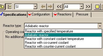
Fro this example we will choose to simulate an adiabatic reactor.
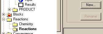
The next thing to do is enter the reaction data. Double click on the "Reactions" folder in the input section of the Flow Sheet window. The menu now present should have "Chemistry" and "Reactions." Click on "Reactions" to bring up a window where you can enter information about the reactions. Click on the "New" button in that window.
By selecting "New" we are telling Aspen that we want to define a set of reactions that is going to take place in one of the units in the model. From the "Object Type" menu that just appeared, select "Powerlaw." Next, name your reaction set in the "Create" window that just appeared. This example will use the default name, "R-1." We can then edit the reaction window for the first reaction to make it look like.
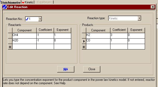
This page represents the stoiciometry for the reaction
The numbers in the "Coefficient" column represent the stoiciometry of the reactions. The "Exponent" column contains the power law exponents in the equations. For example, in the following equation:
only methane appears to affect the rate; therefore, it gets a "1" in the "Exponent" column while all other compounds get a zero.
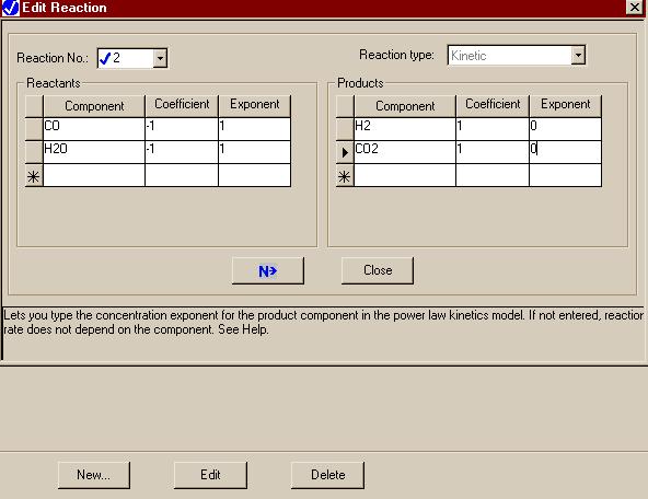
Use of the "New" button at the bottom of that window allows us to enter similar data for the second reaction:
|
|
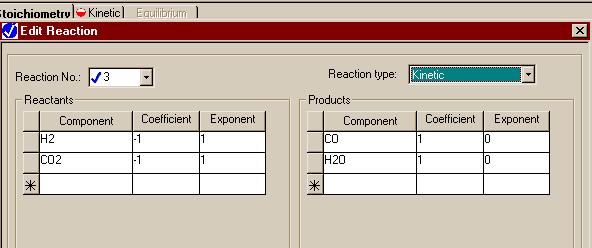
Finally, here is the window for the third reaction.
|
|
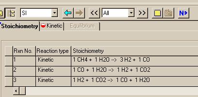
When you press the "Next" button, you will be able to see the reactions that you have specified. Here is what you get after doing that following the specification of the 3rd reaction:
Now that this is complete, we need to enter the kinetics data for the three reactions. To do this, click on the "Next" button shown in the above figure and edit the file to look like:
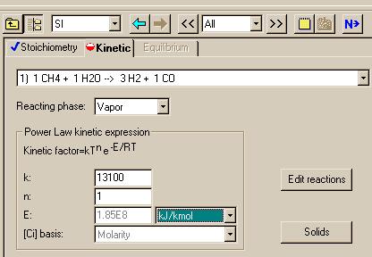 |
Changing to the second reaction in the small window that displays the reaction, allows us to set the next reaction:
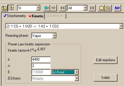 |
Repeating for the third reaction:
 |
This concludes (finally!) the section on entering the reaction data for the system.
The next page to fill specifies the size of the reactor. This window will appear when you click on the "Next" button:
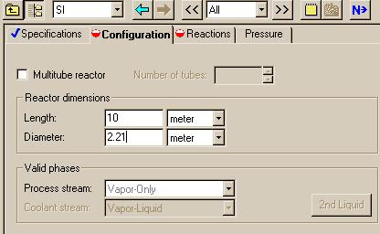
Notice that the reactor diameter is different from the reactor diameter in the Matlab example. In the Matlab example, the porosity (phi) is 0.48. To account for the porosity, we use the following relation:
		     pi*(Deff)2     phi*pi*D2
		     ---------  =  ----------
		         4             4
or
Deff = sqrt(phi) * D = sqrt(0.48)*3.19 m = 2.21 m
The next window allows us to specify that we want to include the "R-1" reaction set. It should look like this after we finish.
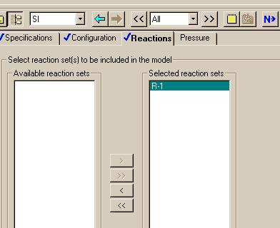
Note that the "Reactions" are now complete and clicking on the "Next" button brings up the welcome message:
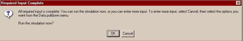
Select "Cancel" before you run the model so that you may first save the file. It is best to save it in the back up mode.
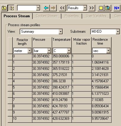
We are now ready to execute the system. To do this, first "View" the Control Panel and execute with the "Run" button under the "Run" menu.. When Aspen has finished the calculations, pull up the results under the Data menu: Results Summary: Streams to see:
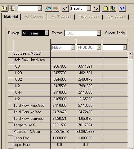 |
You can change the "View" to see changes in mol fractions of the compounds:
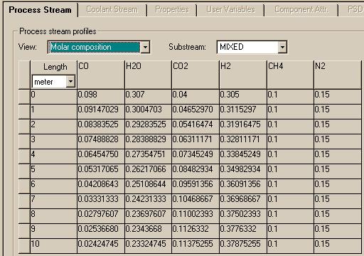
These results compare well to those found using Matlab.
To allow you to see how the results compare, the following graph compares the mole fraction of water in both systems. The dotted blue line represents the Matlab data while the solid red line corresponds to the Aspen data.
|
|