Fri. Jan 20: Short article, “Hydroxyapatite Composite Biomaterials” from AZoM.com

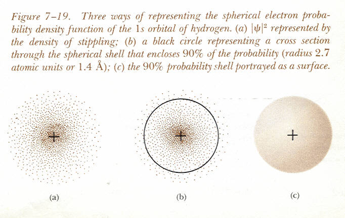
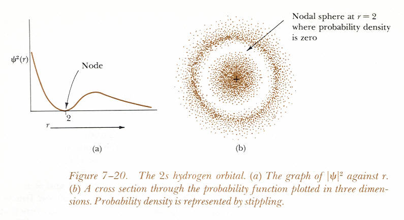
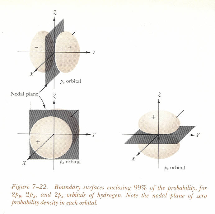
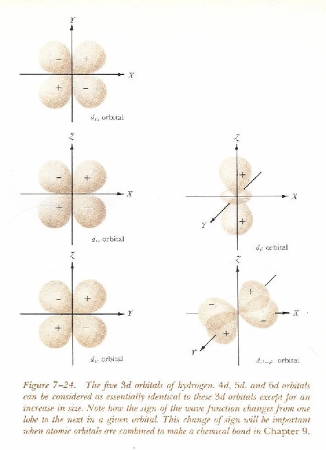
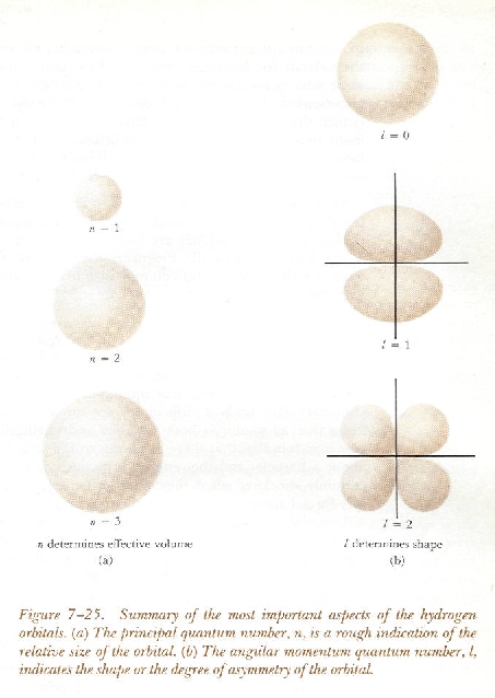
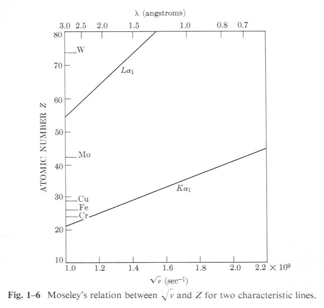
Mon. Jan 23: Bohr orbitals: 1s, 2s, 2p, 3d, Effect of n & l quantum numbers hybrid orbitals sp3, sp2, sp as well as Hydrogen-like energy levels and Moseley's Law

Wed. Jan 25: Hydrogen bonds from chemguide.co.uk

Fri. Jan 27: Number of elastic constants for each crystal system from Dieter and Dependence of Material Properties on Crystal Direction from Metals Handbook as well as Tetrahedral and octahedral interstitial sites in FCC Bravais lattice and also BCC case. More interstitials in FCC, HCP, BCC lattices from GAMGI.ORG.

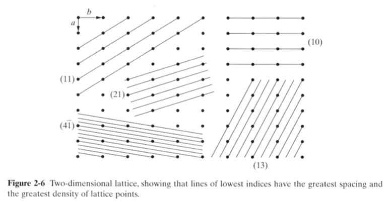
Mon. Jan 30: Examples of Miller indices and plane spacing in two spatial dimensions from Cullity.

Wed. Feb 1: Article from the ASM book Thermal Properties of Metals on thermal expansion.

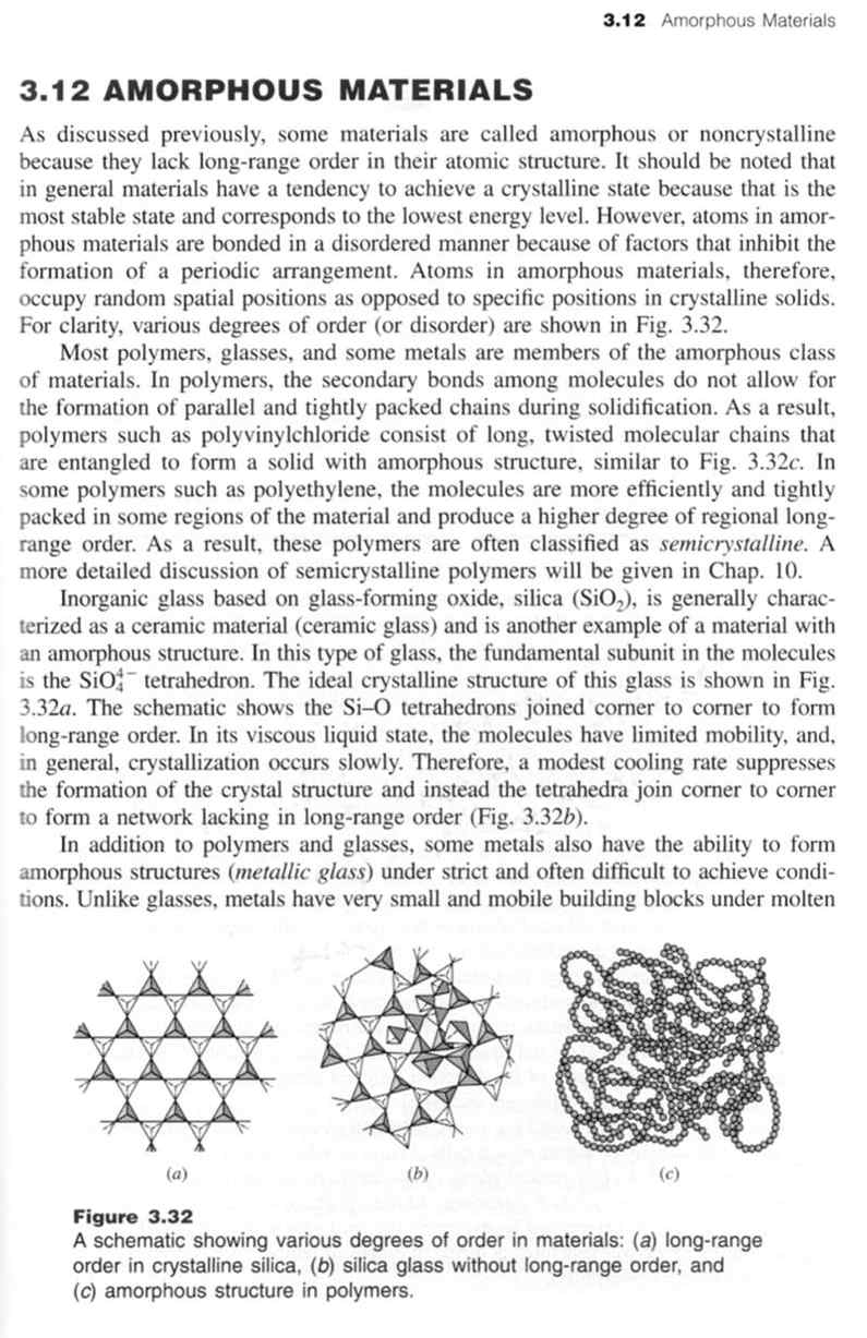
Fri. Feb 3: New section 3.12 in 4^th edition of the text, first and second pages, about amorphous materials.

Fri. Feb 10: Transmission electron microscope (TEM) photos of dislocation loops caused by shear strain acting on crystal defects. The loops tend to lie in certain crystallographic planes and the sides of each loop tend to lie along certain crystallographic directions. In each loop, one pair of opposite sides are edge-type and the other pair are screw-type. Also, see schematic drawings of three-dimensional coherent, semi-coherent & non-coherent precipitates in a crystal.

Mon. Feb 13: For self-diffusion in polycrystalline Ag, grain boundaries dominate below about 950 deg.K (lower activation energy and higher diffusivity) while lattice diffusion dominates above that temperature (higher activation energy and lower diffusivity). See plot. This type of behavior is common in nearly all polycrystalline materials. Free surface diffusion is faster than along grain boundaries and has even lower activation energy. See schematic diagram where the horizontal axis is normalized for various alloys by plotting melting temperature over ambient temperature.

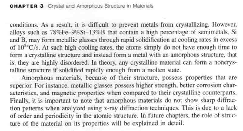
Wed. Feb 15: Comparison of the normal and lognormal distributions, both with standard deviation=1 and a graph of the error function and some reference information about it.

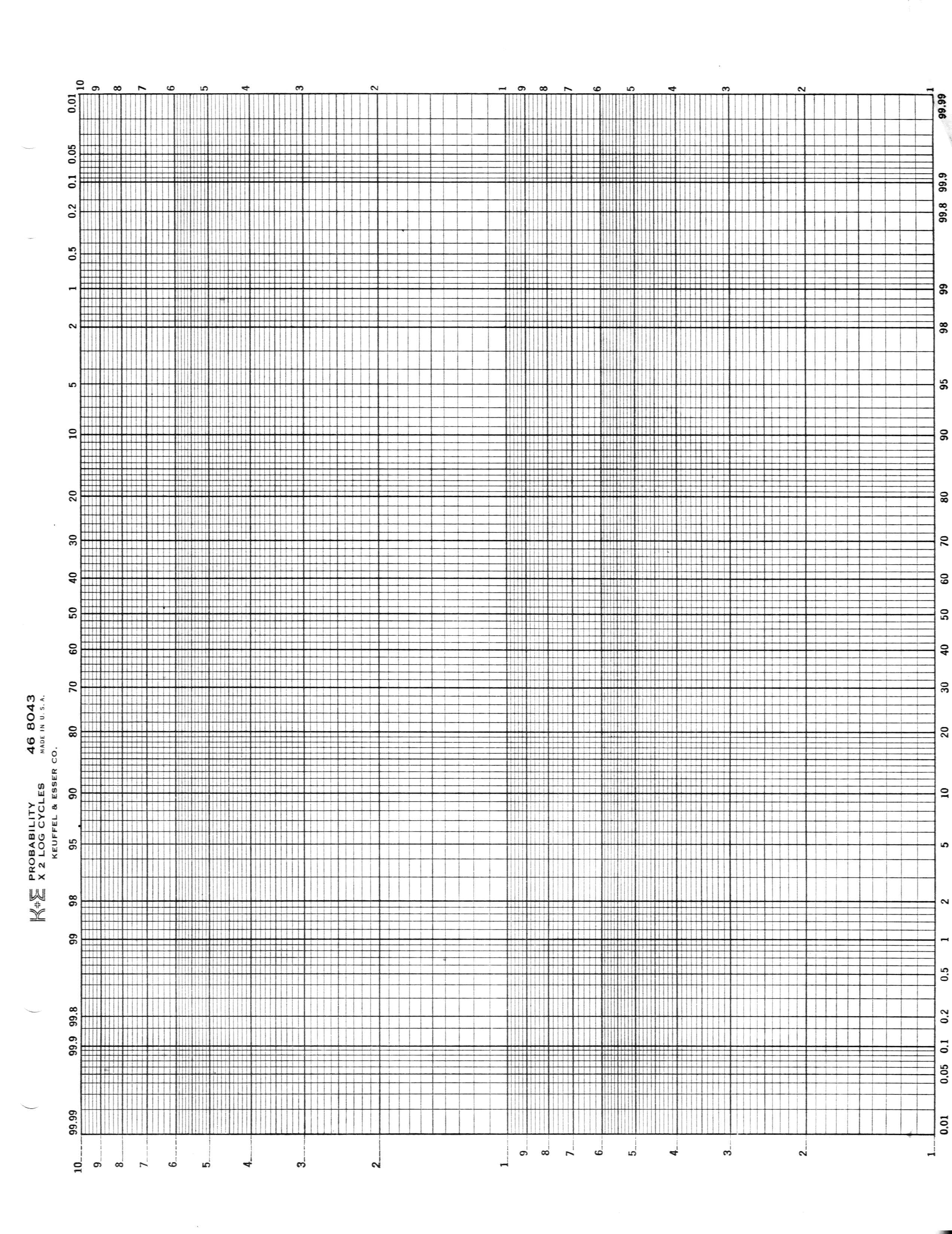
Fri. Feb 17: Log-normal graph paper, for use with "censored" data. Example of thermally activated failure: estimation of MTTF for two parts failed out of 100.

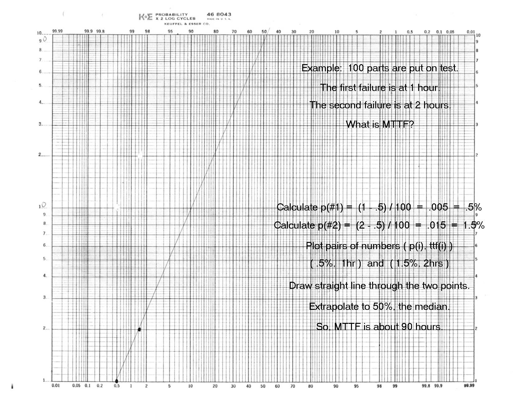
Mon. Feb 20: Here is a link to the NIST/SEMATECH Engineering Statistics Handbook, section 8.2.2.1 Probability Plotting . The paragraph Plotting Positions was mentioned in class. Also, in case you'd like to calculate the error function ERF and/or its inverse ERFINV using Excel spreadsheet functions NORMSDIST and NORMSINV, just copy and paste the right hand side of the equations below into your spreadsheet and replace X with a spreadsheet column & row.

ERF[ X ] = 2*NORMSDIST( X*SQRT(2) ) - 1

and ERFINV[ X ] = NORMSINV( (X+1) / 2 ) / SQRT(2)

Mon. Feb.27: See summary of scanned probe microscopes which all depend on piezoelectric actuators as well as comparison of SEM and TEM.

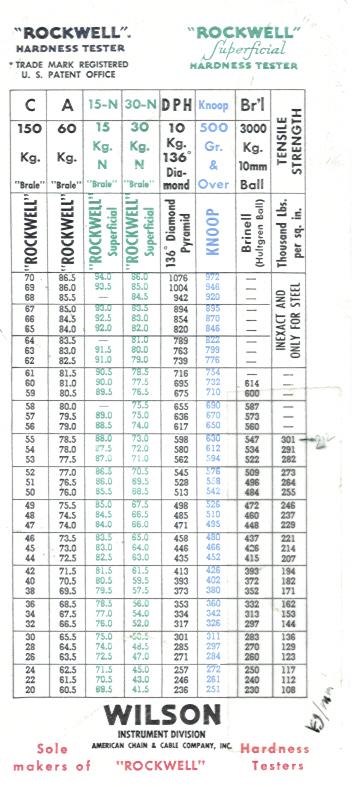
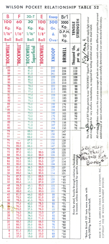
Mon. Mar.6: See hardness conversion tables, part 1 and part 2, from Wilson Instrument. These can be used to convert between hardness measurements of various types and also, for steel, to convert hardness readings into ultimate tensile strength. Note that the units for Knoop, Brinell and DPH (Vickers) hardness are all Kg per square mm, while the units for tensile strength are K psi. Rockwell hardness numbers don't have explicit units. Two other useful references about hardness testing are from the Univ. of Maryland and from the Gordon England company.

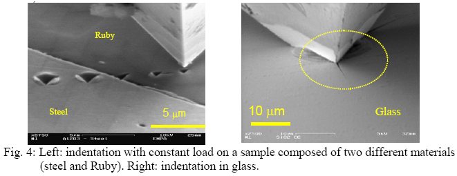
Wed. Mar.8: Some interesting links about nano- and micro-indentation testing: www.microphotonics.com/nht.html note the numerous applications of nano-indentation testing and the equipment specifications; www.mtsnano.com/pdf/appnote_fracturetough.pdf a method of fracture toughness measurement for brittle materials; www.mtsnano.com/pdf/appnote_rbc.pdf indentation and imaging of red blood cells with one instrument; indentation in an SEM by Mazerolle, Rabe, Varidel & Breguet :

Mon.Mar.13 – Fri. Mar.17 Spring break.

Mon. Mar.20: In case you haven’t seen the movie, at least you can read the metallurgical failure analysis report about the RMS Titanic.

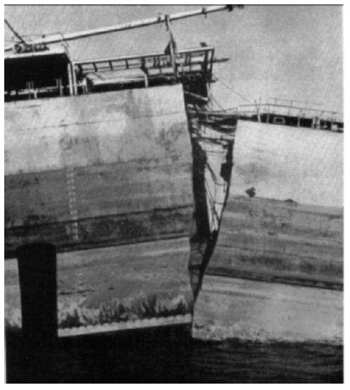
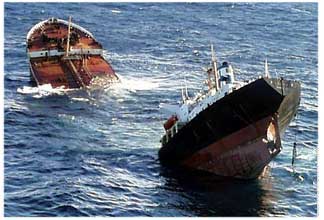
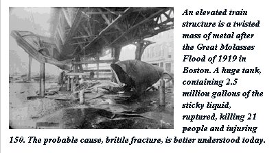
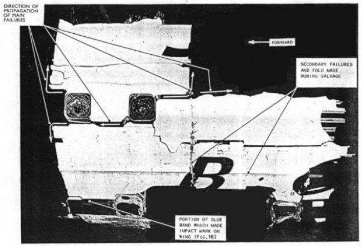
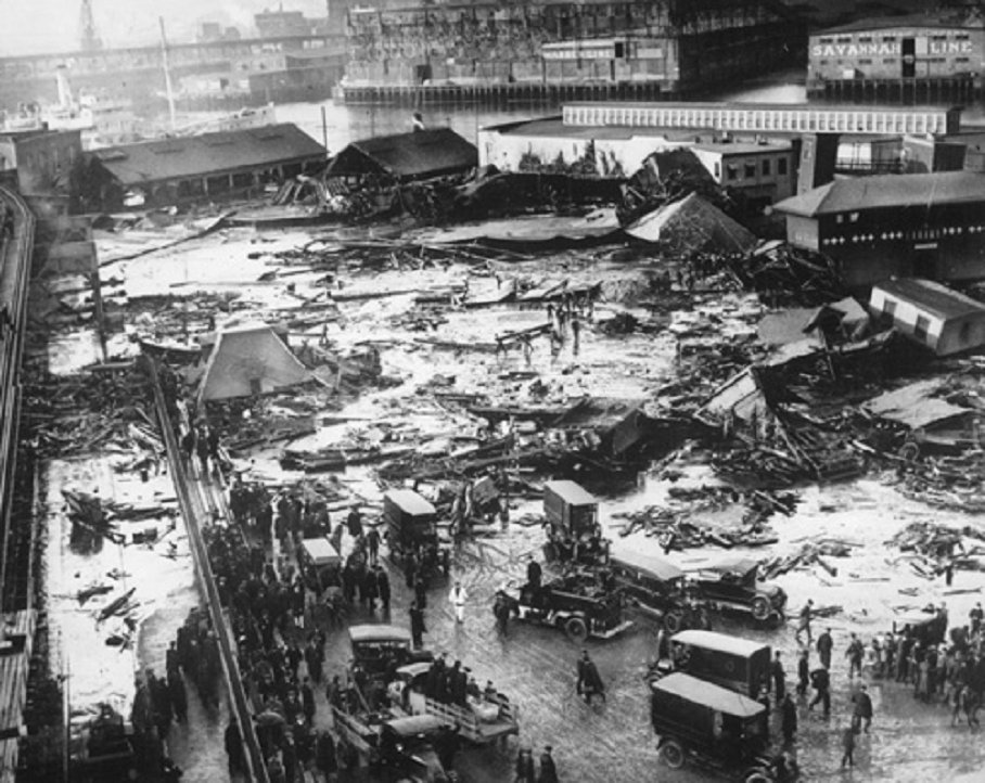
Wed. Mar.22: A few photos of cracked Liberty ships from the bad old days before the development of fracture mechanics. Another of those plus in 2002 sinking of the Prestige. A photo of the world's first model of jet airliner, the De Havilland Comet which was prone to sudden fracture of the fuselage and loss of the entire plane due to growth of cracks from rivet holes near windows and hatchways. See description. 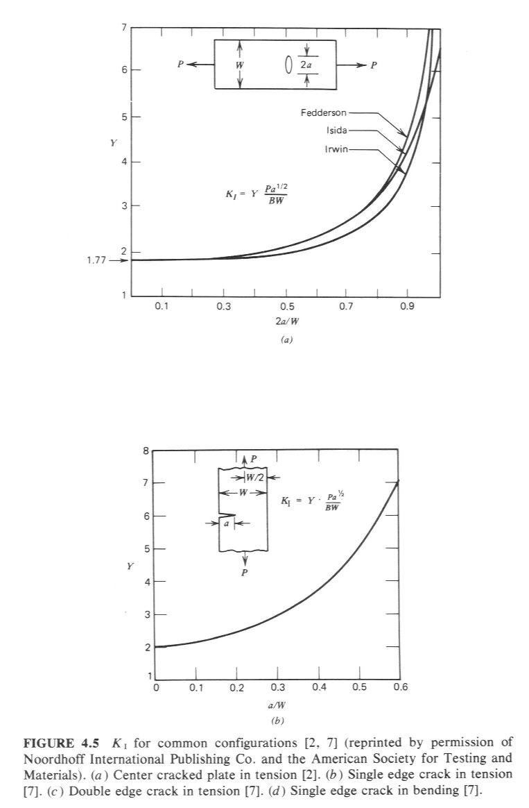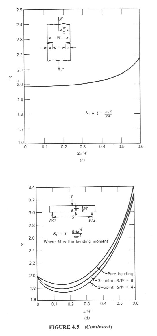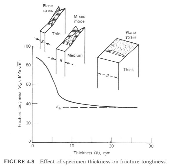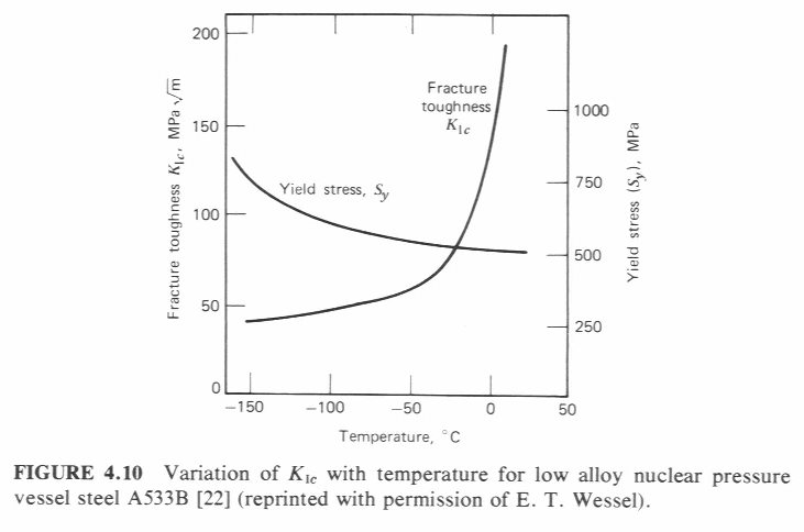And one more fracture catastrophe, the Boston Molasses tank disaster of 1919 and a second view of that.

Also, from Fuchs & Stephens, graphs of stress intensity as a function of crack length for center cracked & single edge notched strips in tension as well as double edge notched strip in tension & single edge notched strip in bending. Also a graph showing the effect of specimen thickness on fracture toughness and a graph showing variation of Kic with temperature.

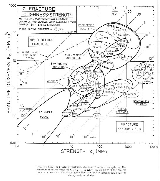
Fri. Mar.24: A chart from Ashby, Kic as a function of yield stress for a wide variety of solid materials. This is especially useful for comparing critical crack sizes among the various materials.

Mon. Mar.20: Here is an example of a good Msci 301 term paper from back in 2004, tied for best in class with a score of 24 out of 25. The format is JPG files stuffed into an MS Word document. Also, be sure to correct two errors in your text: 3^rd edition equations 6.23 & 6.24 and in 4^th edition equations 7.21 & 7.22 . The square bracket ] should be before (20 .

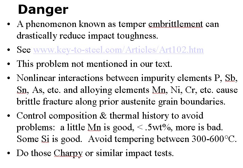
Fri. Mar.31: Our text discusses tempering and other heat treatments for steel in considerable detail but never mentions temper embrittlement. This embrittlement is a big problem. For details, see an article on the subject at www.key-to-steel.com/Articles/Art102.htm . This web site also includes has a wealth of other information about steel, mechanical testing, fracture mechanics, fatigue, etc. Also a brief summary of temper embrittlement by your instructor.

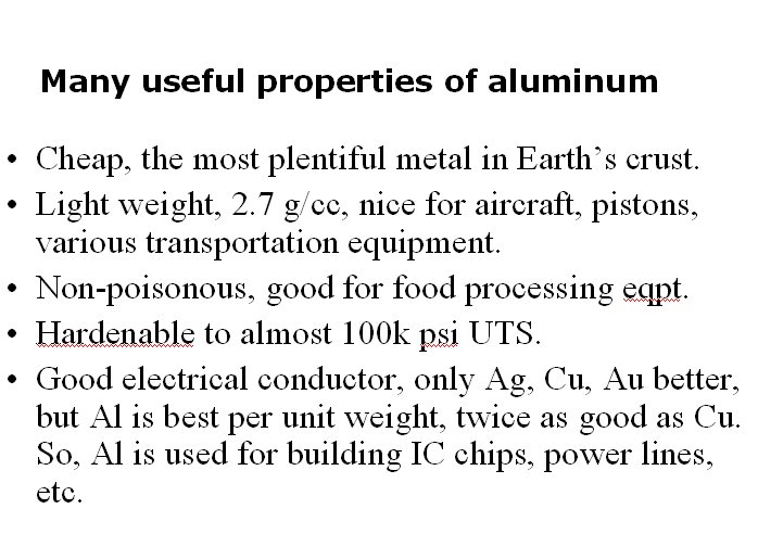
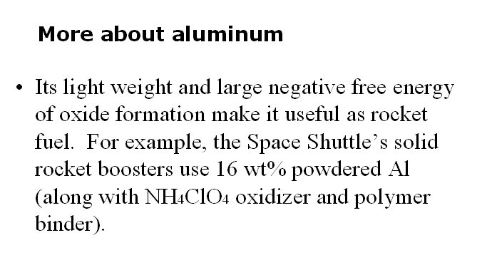
Mon. Apr.3: A few slides from today’s lecture about the properties of aluminum alloys: slide 1, slide 2, slide 3, slide 4.

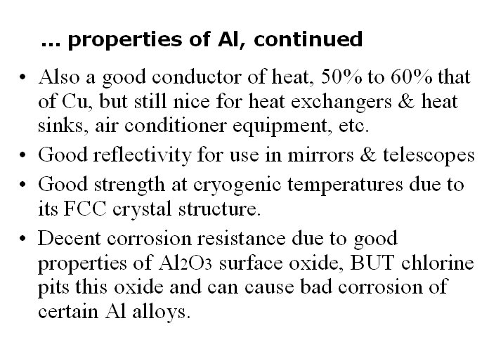
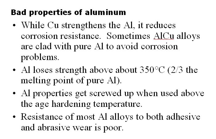
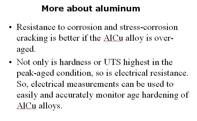
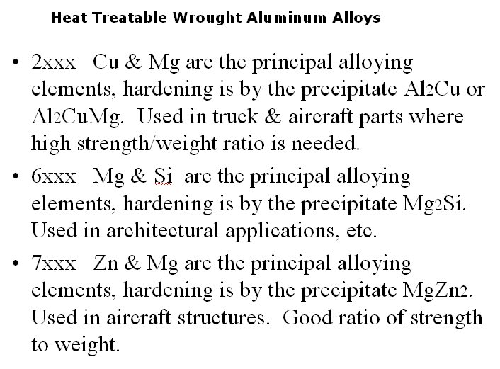
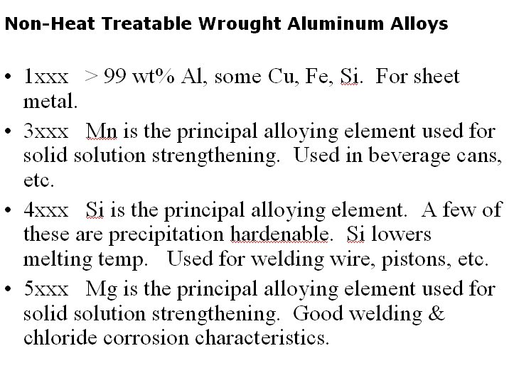
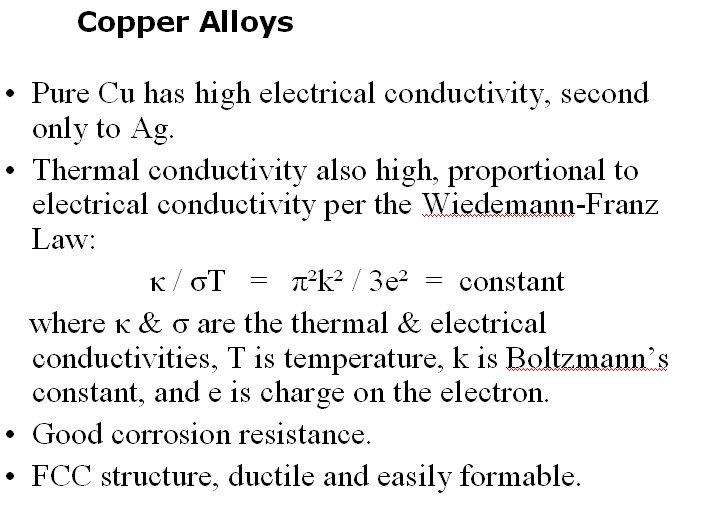
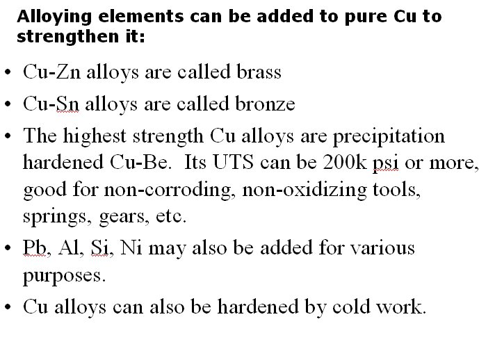
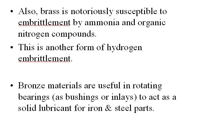
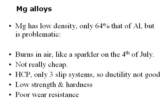
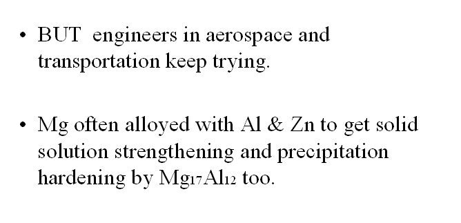
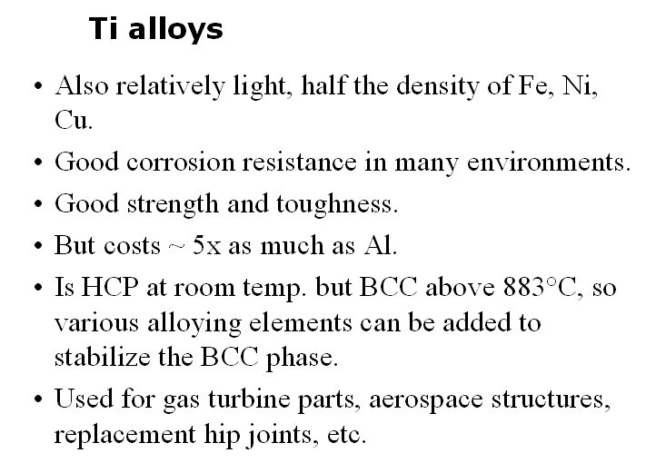
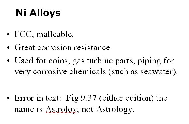
Wed. Apr.5: One more slide about aluminum properties: slide 5 and a summary of the types of wrought aluminum alloys, some heat treatable and some not. A reading assignment about the earliest aluminum alloys, the dawn of nano-engineering: The First Aerospace Aluminum Alloy: The Wright Flyer Crankcase by Frank Gayle of NIST. Finally, a few slides summarizing the properties and uses of Cu alloys: slide_A, slide_B, slide_C, slide_D; Mg alloys: slide_E, slide_F; as well as Ti_alloys and Ni_alloys.

Fri. Apr.7: no class, spring recess …

Mon. Apr.10: As discussed in class, the term paper due date has been changed from Fri. 4/14 to Mon. 4/17. There will be a short homework assignment due on Fri. 4/14.

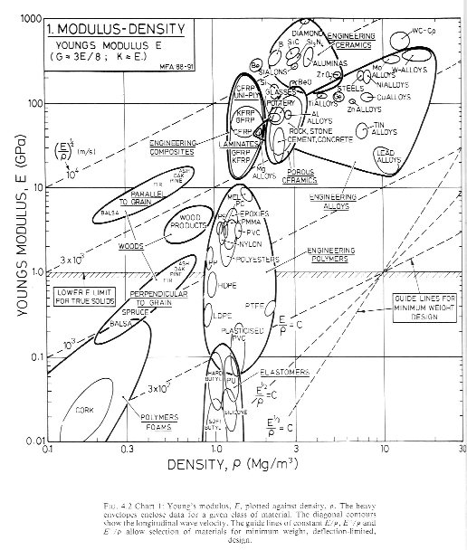
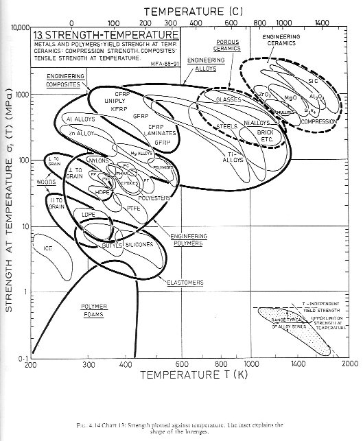
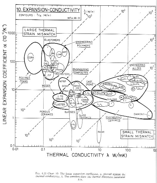
Wed. Apr.12: To compare various properties of ceramics with those of metals (and other materials) see charts by Ashby: elastic modulus vs. density, strength vs. temperature, and thermal expansion vs. thermal conductivity . In Ashby’s graph of thermal expansion, α, versus thermal conductivity, λ, note the ratio λ/α which he refers to as the thermal distortion parameter. Better still, one will find in the literature a thermal shock resistance, TSR, defined as TSR = λσ/αE where σ is the strength (fracture or yield) and E is the elastic modulus. TSR can be especially important for brittle materials subject to rapid heating.

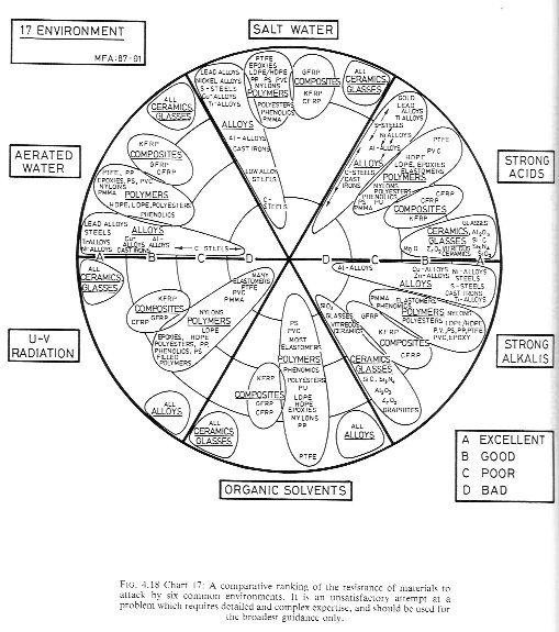
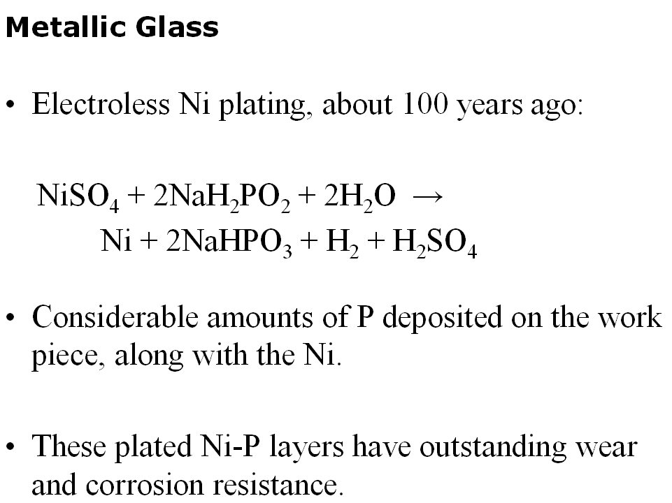
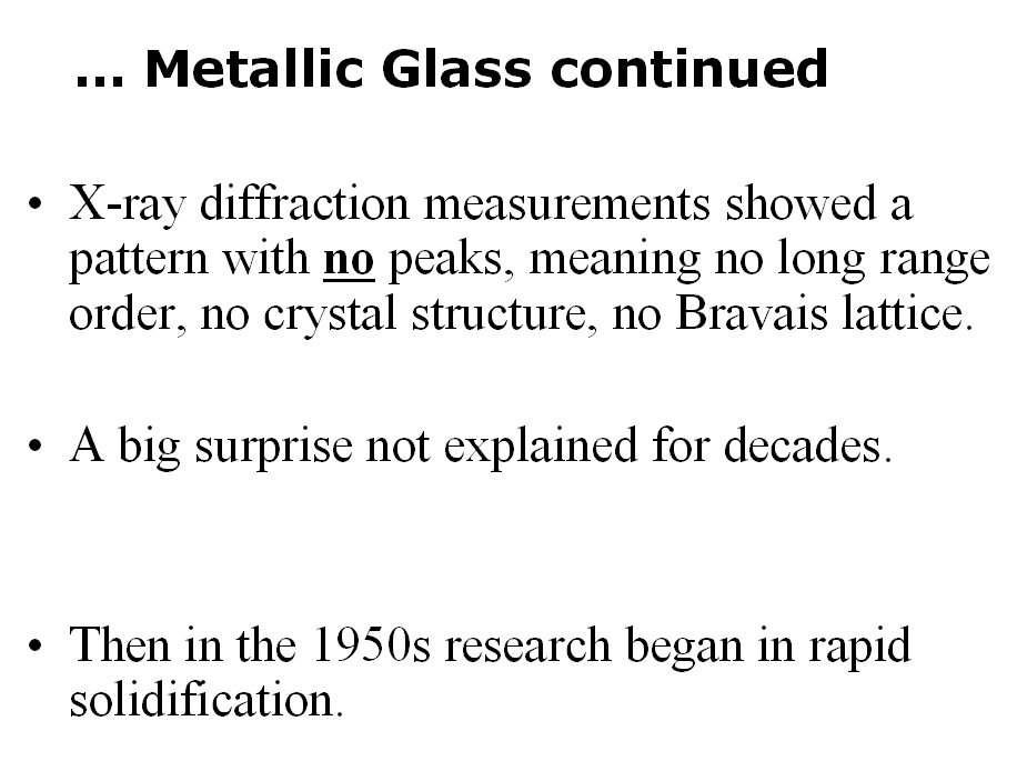
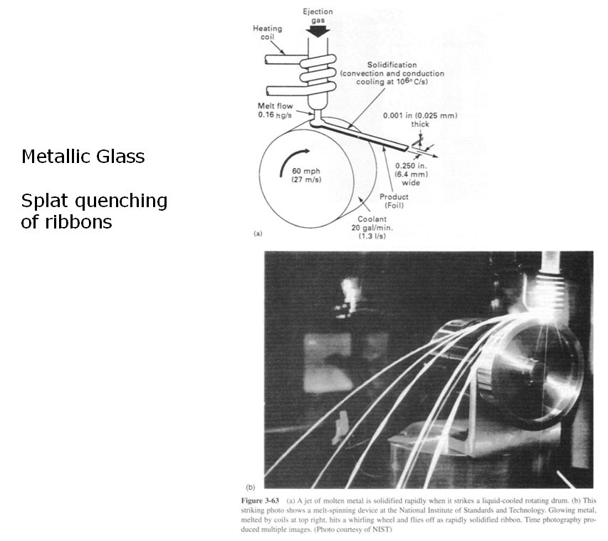
Fri. Apr.14: Another Ashby chart summarizing corrosion of materials in various chemical environments. Note Ashby’s disclaimer in the caption to this figure. Although he does not mention it, many ceramics can be severely affected by fluorides such as hydrofluoric acid. There was also a discussion of metallic glass. The first metallic glass was produced about 100 years ago by an electroless plating process, more recently by splat quenching. See slides (1), (2) & (3). Splat quenched alloys are typically composed of a diverse combination of elements: transition metals such as Ni & Fe, nonmetals such as B & P, perhaps alloyed with other metals such as Al. The atoms are chosen so that their sizes vary over a wide range and so that there is a combination of covalent and metallic bonding between nearest neighbors, all of which slows the crystallization process during cooling. Metallic glass alloys have properties intermediate between those of metals and glassy ceramics – good strength and fracture toughness - both!, good corrosion resistance, good wear resistance, especially large elastic limit, etc. Recently, some alloys such as Zr₄₁Ti₁₄Cu₁₃Ni₁₀Be₂₂ and ZrTiCuNiAl have been cast into molds and remained in the glassy state.

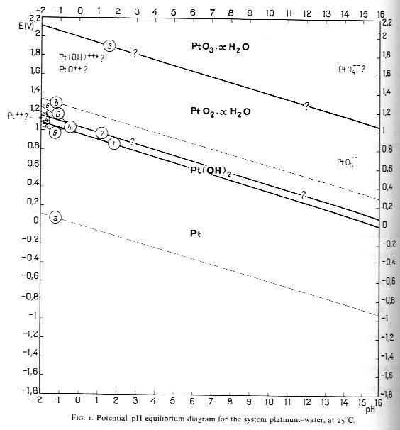
Mon. Apr.17: Pourbaix potential-pH diagrams for both Al and Pt were discussed in class but not mentioned in the Smith text. Areas in each of these diagrams fall into one of three categories, depending on the behavior of the material: either corrosion, passivation or immunity. Immunity occurs at low potentials, where the reaction M⁺ + e^- → M would cause metal ions to be plated from solution onto the anode. Passivation occurs in areas of the Pourbaix diagram where insoluble oxide or hydroxide films form and protect the metal from corrosion. Corrosion occurs elsewhere in the diagram as metal ions or soluble metal-oxygen-hydrogen compounds go into aqueous solution.

In the Al-water diagram, for example, corrosion occurs in a large area where pH>8.6 and E>-2 or so where the aluminate ion AlO₂^- goes into aqueous solution. Al corrosion also occurs in a large region where pH<4 and E>-1.65 (roughly), where Al⁺⁺⁺ or Al⁺ ions go into solution. Passivation by hydrated Al₂O₃ occurs in a vertical band on the diagram where 4<pH<8.6 and E>-2 (roughly). Al is immune toward the bottom left part of the diagram, below diagonal line 2.

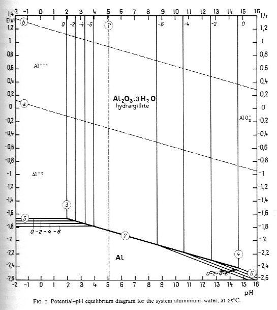
While Al is quite corrodible, Pt is not. Referring to the Pt-water diagram, corrosion occurs only in a small region close to pH=-2 and E=1.1. Over a large area in the upper part of the diagram Pt is passivated by insoluble PtOH₂ or hydrated PtO₂ or PtO₃. And over a large area at the bottom of the diagram Pt is immune.

These E-pH diagrams are valid ONLY for the simple systems of metal in water wherein a limited number of chemical reactions are possible, obviously all involving metal, hydrogen and oxygen. If complexing agents such as chlorine or sulfur are present, additional chemical reactions are possible and the Pourbaix diagrams can change substantially. A classic example is corrosion of Al in the presence of chlorides. These attack the passive Al₂O₃ layer, cause pits to form in it, and expose the underlying metal to rapid corrosion. This action causes the region of passivation on the E-pH diagram to be much smaller.

Wed. Apr.19: Pourbaix E-pH diagrams usually include two diagonal lines:

Line (a) from (E,pH)=(-.059,0.0) to (-.59,10.) which results from the hydrogen evolution reaction 2H⁺ + 2e^- = H₂ and corresponding Nernst equation E=0.0-.0591*pH. Below this line, H₂ is given off and the solution becomes more alkaline. This chemical reaction can be written in slightly different form (adding 2OH^- to both sides) as 2H₂O + 2e^- = H₂+ 2OH^- which could be described as the reduction of water.
Line (b) from (1.23,0) to (.64,10) which results from the oxygen reduction reaction 2H₂O = O₂ + 4H⁺ + 4e^- and corresponding Nernst equation E=1.228-.0591*pH. Above this line, O₂ is given off and the solution becomes more acidic. This chemical reaction can be written in slightly different form as O₂ + 2H₂O + 4e^- = 4OH^-.

In between these two lines water is stable. Both of the above chemical reactions are discussed in the Smith text and listed in Table 12.1 (3^rd Ed) or 13.1 (4^th Ed).

Other lines also appear on the Pourbaix diagrams, as follows. Vertical lines correspond to chemical reactions which depend on pH but not potential. An example is Al₂O₃ + H₂O = 2AlO₂^- + 2H⁺ . This is independent of potential because electrons e^- do not appear in the reaction equation. Horizontal lines correspond to chemical reactions which depend on potential but not pH. An example is Al = Al⁺⁺⁺ + 3e^- . This is independent of pH because the H⁺ ion does not appear in the equation. Other reactions mentioned above include both e^- and H⁺ and so are functions of both E and pH.

Small integer numbers near lines on the Pourbaix plot are the base 10 logarithm of the concentration of the soluble species in solution. As a crude rule of thumb, for values < -6 not much corrosion is going on.

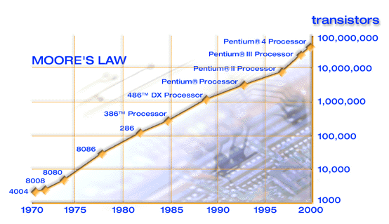
Fri. Apr.21: In the late 1960's Gordon Moore at Fairchild Instrument noticed that the complexity of integrated circuit (IC) chips was doubling every year or so. This trend has persisted in the semiconductor industry for decades (see trend for Intel processors). Similar trends exists for other companies and for both memory and logic circuitry, due in no small part to thousands of engineers working to understand the effects of electric currents, mechanical stress, temperature and impurities on various metals, insulators and semiconductors used in building those chips.

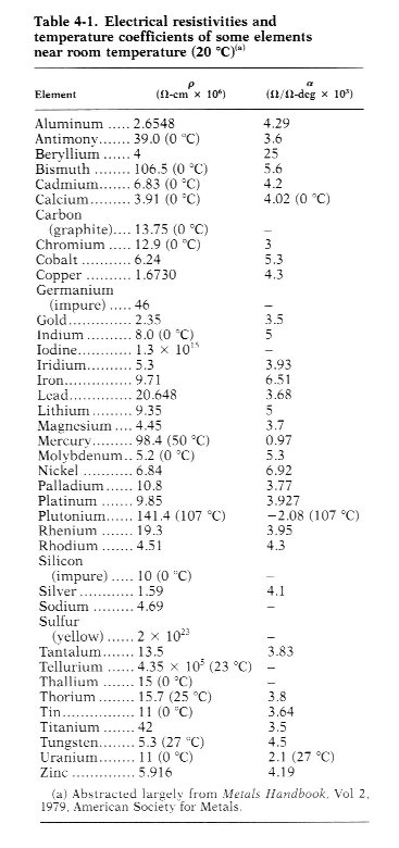
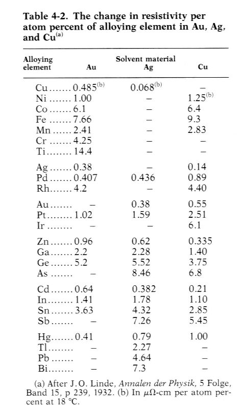
Resistivity r and temperature coefficient of resistivity a (or TCR) for forty pure elements are shown in a table from Pollock. The effects of various solute atoms on the resistivity of Au, Ag and Cu are tabulated here.

Mon. Apr.24: Besides IC chips, resistors have many other applications, including

1) Temperature measurement, using r (T) = r 0C (1 + a *T) per Smith eqn. 13.8 . Pt works well in this application.

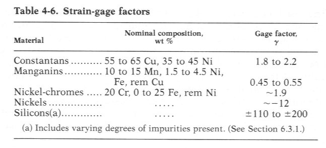
2) Strain measurement: if one starts with the equation for resistance R = r l /A (Smith eqn. 13.2), then takes the total derivative D of both sides and divides the result by the original equation, the result is D R = (AD l - l D A)/ l A . Noting that, due to constant volume, strain e = D l /l = -D A/A (Smith eqn. 5.4) it can be shown that D R/R = 2e for "normal" metals. Here, D R is just the change in resistance due to strain. More generally, a material’s "gage factor" is defined as g = D R/Re . See values for various materials.

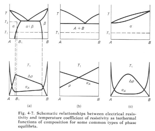
3) Phase diagram determination: Temperature coefficient of resistivity a and resistivity r depend on alloy composition as shown in a figure by Pollock.

4) Heat treatment of precipitation hardening alloys. - Maximum hardness, yield and tensile strength occur in precipitation-hardening alloys when the number of GP zones is greatest. At this same point electrical resistivity is also greatest. So, an electrical resistance method is used commercially to control heat treatments of such alloys, particularly aluminum alloys for aircraft. In many cases these are aged just past the peak-aged condition to improve corrosion resistance at the expense of a relatively small decrease in strength. This method is much quicker, easier and more accurate than hardness testing, electron microscopy, and other alternatives.