Several Matlab functions have been written for help with non-ideal multicomponent simulations. The following table lists the functions that have been written and tested to date:
|
|
|
|
|
|
|
>> [t,ys]=bubptg(p,xs) |
|
|
|
>> buberg(3,amipa) |
|
|
|
>> [p,ys]=bubtpg(t,xs) |
|
|
|
>> buberg2(3,amipa2) |
|
|
|
>> gams=marg1(xs) |
|
|
|
>> minvle(Amarg) |
|
|
|
>> XG=terf1(amipa) |
The ternary sytem: acetone, methanol, isopropyl alcohol will be the example that we use to demonstrate the programs. Data for this system was reported by Freshwater and Pike in the J. Chemical Engineering Data 12 page 179 1967. Two tables of ternary data were presented for this system. In the first set, the pressure was fixed at 760 mmHg and in the second set the temperature was fixed at 55C. The data for each set stored in a text file that was then read into a Matlab session. The isobaric data was stored in a file called amipa. It looked like the following when listed in Matlab:
       x1        x2        y1        y2    T in C   p in mmHg
    0.0360    0.5460    0.1050    0.6750   69.3000  760.0000
    0.0930    0.5230    0.2390    0.5810   66.8400  760.0000
    0.1360    0.2980    0.3350    0.3690   68.8300  760.0000
    0.0370    0.1120    0.1210    0.1699   76.9700  760.0000
    0.8708    0.0761    0.8866    0.0912   56.3200  760.0000
    0.5459    0.2693    0.6680    0.2569   58.4500  760.0000
    0.3555    0.1917    0.5780    0.2096   63.6500  760.0000
    0.0520    0.0287    0.1606    0.0485   77.4100  760.0000
    0.1324    0.2635    0.3218    0.3391   69.2300  760.0000
    0.0950    0.4453    0.2306    0.5135   68.1800  760.0000
    0.0601    0.8993    0.1300    0.8556   63.1000  760.0000
    0.1231    0.6965    0.2469    0.6776   63.2700  760.0000
    0.3948    0.4841    0.5346    0.4237   58.4300  760.0000
    0.2635    0.3920    0.4576    0.3861   62.9500  760.0000
    0.3089    0.1895    0.5465    0.2040   64.6500  760.0000
    0.0820    0.5602    0.1955    0.6259   66.7900  760.0000
    0.3167    0.4201    0.4923    0.4023   61.2900  760.0000
    0.3732    0.5910    0.4982    0.4923   57.5400  760.0000
    0.4062    0.5355    0.5315    0.4490   57.5600  760.0000
    0.4089    0.0351    0.6596    0.0552   64.7300  760.0000
    0.4854    0.1379    0.6768    0.1480   61.7700  760.0000
The program terf1 was used to convert this data into an array containg the liquid mols fractions of all the compounds followed by the liquid activity coefficients by the following definition:
where: yi is the vapor mol fraction of compound i
xi is the liquid mol fraction of compound i
P is the total pressure and
pi*(T) is the vapor pressure of compound i.
Here is a listing of the conversion program:
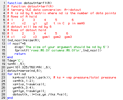
This program was used to create the array XG1 from the isobaric data set in amipa and the array XG2 from the isothemal data set in amipa2. Property data for the three compounds (including "Mass & Energy" balance data) must be set with start301 before it can be executed. Here is a listing from Matlab of XG1:
       x1        x2        x3      gam1       gam2     gam3
    0.0360    0.5460    0.4180    1.8890    1.0322    0.8961
    0.0930    0.5230    0.3840    1.7991    1.0194    0.8880
    0.1360    0.2980    0.5660    1.6191    1.0526    0.9086
    0.0370    0.1120    0.8510    1.6747    0.9526    1.0295
    0.8708    0.0761    0.0531    1.0089    1.6763    1.2796
    0.5459    0.2693    0.1848    1.1280    1.2222    1.1251
    0.3555    0.1917    0.4528    1.2615    1.1366    1.0236
    0.0520    0.0287    0.9193    1.5609    1.0444    1.0441
    0.1324    0.2635    0.6041    1.5776    1.0774    0.9586
    0.0950    0.4453    0.4597    1.6286    1.0049    0.9947
    0.0601    0.8993    0.0406    1.7087    1.0108    0.7933
    0.1231    0.6965    0.1804    1.5756    1.0266    0.9290
    0.3948    0.4841    0.1211    1.2490    1.1223    0.9542
    0.2635    0.3920    0.3445    1.3786    1.0526    1.0217
    0.3089    0.1895    0.5016    1.3288    1.0758    1.0380
    0.0820    0.5602    0.3578    1.6717    1.0272    0.9477
    0.3167    0.4201    0.2632    1.3032    1.0935    0.9724
    0.3732    0.5910    0.0358    1.2690    1.1078    0.7667
    0.4062    0.5355    0.0583    1.2430    1.1142    0.9654
    0.4089    0.0351    0.5560    1.2085    1.5667    1.0666
    0.4854    0.1379    0.3767    1.1506    1.2022    1.1049
Here is the function used to find the "best" parameters to fit the data in an array like XG1.
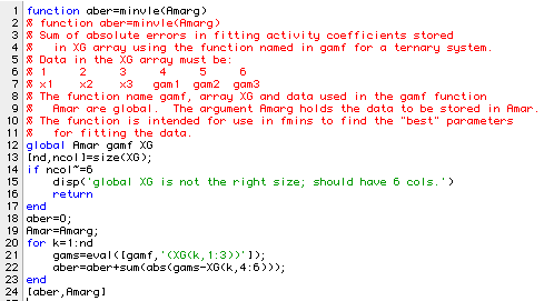
The following session shows a test of this program and the beginning of the execution of fmins to find the "best" values for the parameters to fit the isobaric data:
»global Amar gamf XG
»gamf='marg1';
»XG=XG1;
»minvle([0 0 0])
ans =
   13.7054         0         0         0  <-- sum of abs errors is 13.7
ans =                                          for all zeros in Aber
   13.7054
»fmins('minvle',[0 0 0])
ans =
   13.7054         0         0         0
ans =
   13.7028    0.0003         0         0
ans =
   13.7041         0    0.0003         0
           ....many iterations later.....
ans =
    2.8785    0.6740    0.4880   -0.0639
ans =
    2.8785    0.6740    0.4879   -0.0640
ans =
    2.8785    0.6740    0.4880   -0.0639  <-- sum of abs errors is 2.88
ans =                                         "best" values
    0.6740    0.4880   -0.0639
»Amar1=ans
Amar1 =
    0.6740    0.4880   -0.0639  <-- We will save these best values for
                                 the isobaric data.
»XG=XG2;
»fmins('minvle',Amar1)  <-- Using Amar1 as an initial guess for the
ans =                      isothermal set
    4.4551    0.6740    0.4880   -0.0639
           ....many iterations later.....
ans =
    3.5376    0.6588    0.6060    0.0370
ans =
    0.6588    0.6060    0.0370  <-- Best for isothermal data
»Amar2=ans;
»XG=[XG1;XG2];   <-- Putting in both sets of data
»Amar3=fmins('minvle',(Amar1+Amar)/2)
ans =
    7.0304    0.6664    0.5470   -0.0135
           ....many iterations later.....
ans =
    7.0100    0.6582    0.5409   -0.0142
Amar3 =
    0.6582    0.5409   -0.0142  <-- Best for combined data.
In order to see how well the Margules' activity coefficient model predicts the original data, we need a function to determine the bubble point of our fluid. This requires only a slight modification of the ideal bubble point function: bubpt.
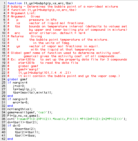
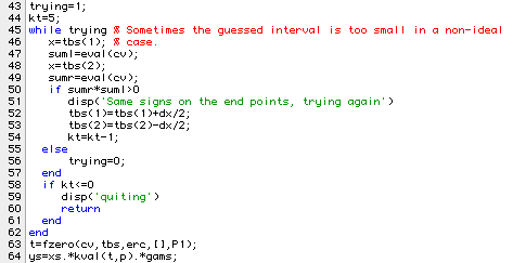
We will see how well we fit the first line of data listed in amipa:
»amipa(1,:)
ans =
    0.0360    0.5460    0.1050    0.6750   69.3000  760.0000
»[t,ys]=bubptg(101.325,[.036 .546 .418])
t =
   69.4051  <-- compared to 69.3
ys =
    0.0984    0.6565    0.2451  <-- exp. values: 0.105 0.675 0.220
Our next program in this section of the notes, mechanizes the process of comparing the bubble points from the experiental data with those predicted by either the ideal program or one using an activity coefficient model such as Margules. Here is the program:
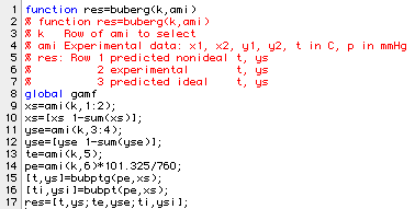
Executing buberg for the first line of data in amipa produces:
»buberg(1,amipa)
ans =
   69.4051    0.0984    0.6565    0.2451  <-- Margules predictions
   69.3000    0.1050    0.6750    0.2200  <-- Experimental
data
   70.4860    0.0577    0.6840    0.2583  <-- Ideal prediction
Two additional programs were written to aid in comparing the isothermal data with the Magules model. The first program: bubtpg determines the pressure and vapor composition for known temperature and liquid composition. Here is a listing:
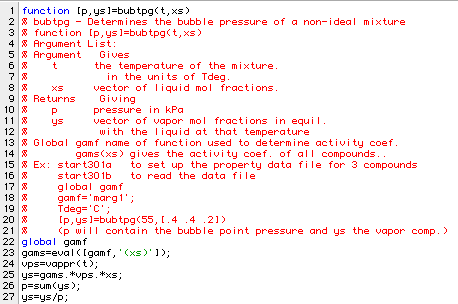
Here is a sample run using data in row 3 of amipa2:
»amipa2(3,:)
ans =
    0.5372    0.3447    0.6480    0.3048   55.0000  695.9000
»[p,ys]=bubtpg(55,[0.5372    0.3447 0.1181])
p =
   93.0284
ys =
    0.6459    0.3091    0.0449  <-- compared to 0.648 0.3048 .0472
»p*760/101.325
ans =
  697.7702  <-- compared to 695.9
The function buberg2 compares each isothermal data set just as buberg did for the isobaric data.
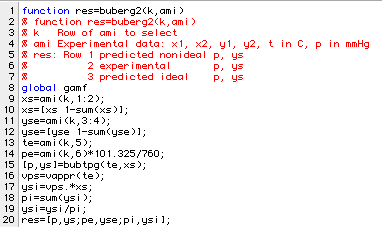
Here is what the program gives for the third row in amipa2:
»buberg2(3,amipa2)
ans =
   93.0284    0.6459    0.3091    0.0449  <-- Margules' prediction
   92.7790    0.6480    0.3048    0.0472  <-- Experimental data
   79.7977    0.6578    0.2962    0.0460  <-- Ideal prediction