We will start with an example from Biegler, L. T., Grossman, I. E., and Westerberg, A. W. Systematic Methods of Chemical Process Design. Example 3.2 in that text shows how to analyze several types of flash separators. The mixture separated includes benzene, toluene and o-xylene. Thus we need property data for those compounds. Using start403a and start403b in Matlab we get a list of our compounds and can set three streams for our separator:
How many streams will there be?3
Here are your compounds' formulae and names:
No. Formula         Name
  1  C6H6           benzene
  2  C6H5CH3        toluene
  3  C6H4CH3CH3-o   o-xylene
In Case 1 we are given the fraction of toluene that should be recovered in the vapor. The text shows how this may be estimated with the assumption of constant relative volatilities among the compounds. We will use trial and error to find this temperature with our Matlab programs.
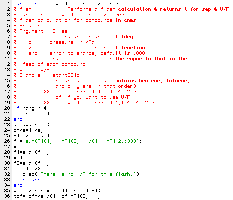
The flsh program can be used to find the fraction of each compound that goes out in the vapor of a flash tank. It also gives the fraction of the feed: V/F that is in the vapor product. Here is a listing of the program.

Here is a program (bgw23) that uses the flsh function to determine the fraction of each compound that goes overhead. The returned value is the error giving the difference between the value for toluene and the specified value: 0.9. The flash is to be carried out at 100 kPa with a feed containing 30 mols benzene, 50 mols toluene and 40 mols o-xylene. Here is the function:

Here is our determination of the flash temperature:
>> bgw32(390)
ans =
    0.1986
>> bgw32(395)
ans =
   -0.0938
>> Tcase1=ssec2([390 395],'bgw32(x)')
Tcase1 =
  393.2825   <-- The text gave 393K
>> flash(Tcase1,100,[30 50 40]/120)
Temperature= 393.28K Pressure= 100.00 kPa V/F=0.8720
Compound      Feed      Liquid    Vapor     K=y/x
 benzene    0.25000   0.09110   0.27333   3.00041
 toluene    0.41667   0.32551   0.43005   1.32115
 o-xylene   0.33333   0.58339   0.29662   0.50844
The liquid mol fractions reported were: 0.089, 0.325 and 0.586. To verify that we really did satisfy the 90% recovery of toluene, we can execute:
>> tof=flsh(Tcase1,100,[30 50 40]/120)
tof =
    0.9534    0.9000    0.7760
We can also use the mass balance modules to see all the flows:
>> ns(1,:)=[30 50 40];  <-- Setting the feed flows
>> sep(tof,1,2:3)       <-- Separating stream 1 into 2 and 3
>> showm(1,2:3,10,3)    <-- Displaying the flows
Compound   Inlet    |            Outlet
   Stream         1 |         2         3   Total
 benzene     30.000 |    28.601     1.399    30.000
 toluene     50.000 |    45.000     5.000    50.000
 o-xylene    40.000 |    31.039     8.961    40.000
Total       120.000 |   104.639    15.361   120.000
All these results agree very well with those found in the text example.
In case 2 we are given the temperature and pressure so our flash function may be used directly to determine the compositions and amounts of the product streams.
>> flash(390,100,[30 50 40]/120)
Temperature= 390.00K Pressure= 100.00 kPa V/F=0.6604
Compound      Feed      Liquid    Vapor     K=y/x
 benzene    0.25000   0.11531   0.31927   2.76875
 toluene    0.41667   0.36639   0.44253   1.20781
 o-xylene   0.33333   0.51830   0.23820   0.45958
The text reports liquid mol fractions of: 0.102, 0.347, 0.55. If we want to see the flows:
>> tof=flsh1(390,100,[30 50 40]/120)
tof =
    0.8433    0.7013    0.4719
>> sep(tof,1,2:3)
>> showm(1,2:3,10,3)
Compound   Inlet    |            Outlet
   Stream         1 |         2         3   Total
 benzene     30.000 |    25.300     4.700    30.000
 toluene     50.000 |    35.067    14.933    50.000
 o-xylene    40.000 |    18.876    21.124    40.000
Total       120.000 |    79.244    40.756   120.000
Here the agreement with the text is less good since they report the liquid (stream 3) flows as: 2.94, 10 and 15.84.
In the third case, we are given the vapor fraction and pressure. Thus we need to estimate the temperature again.

Just as in the other two cases, we can then find:
>> bgw32b(390)
ans =
    0.1396
>> bgw32b(395)
ans =
   -0.1915
>> Tcase3=ssec2([390 395],'bgw32b(x)')
Tcase3 =
  392.1950
>> flash(Tcase3,100,[30 50 40]/120)
Temperature= 392.20K Pressure= 100.00 kPa V/F=0.8000
Compound      Feed      Liquid    Vapor     K=y/x
 benzene    0.25000   0.09852   0.28788   2.92208
 toluene    0.41667   0.33981   0.43588   1.28271
 o-xylene   0.33333   0.56167   0.27624   0.49181
>> tof=flsh(Tcase3,100,[30 50 40]/120)
tof =
    0.9212    0.8369    0.6630
>> sep(tof,1,2:3)
>> showm(1,2:3,10,3)
Compound   Inlet    |            Outlet
   Stream         1 |         2         3   Total
 benzene     30.000 |    27.636     2.364    30.000
 toluene     50.000 |    41.845     8.155    50.000
 o-xylene    40.000 |    26.520    13.480    40.000
Total       120.000 |    96.000    24.000   120.000
These results are much closer to those found in the text than for Case 2.
Example 7.3 in BGW shows a flash of three compounds that are non-ideal: methanol, propanol and acetone. It gives a relation to find the excess Gibbs energy so we can determine the activity coefficients of each compound. The expression is:
GE/RT=-0.753x1x2 + 0.6495x1x3 + 0.557x2x3
The following Maple sessions were used to check the values reported for the activity coefficients derived using eq. 7.14 in BGW.
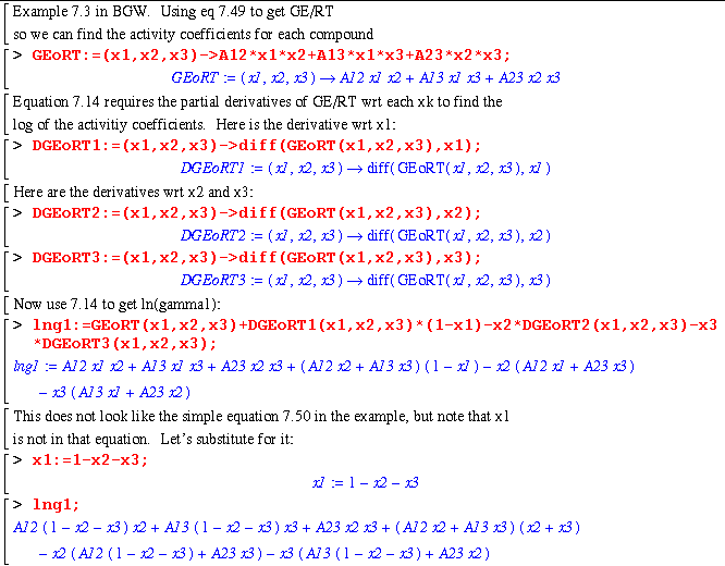
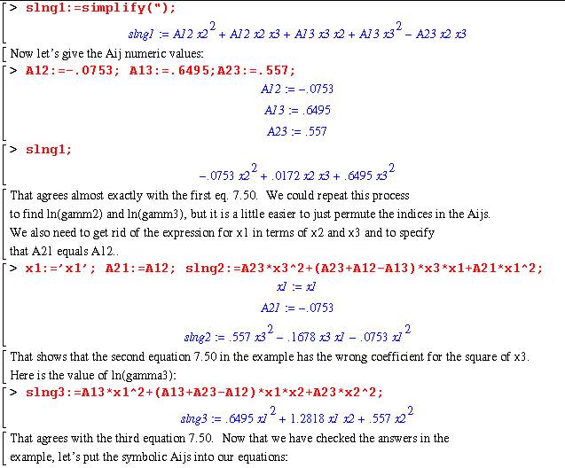
That gave the value of the natural log of the activity coefficient for methanol in the mixture. If we substitute the values given for the Aij into this, we can check the values found in the example.
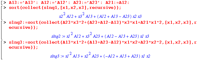
Finally, we should go back to the symbolic form for all the activity coefficients:
Now we need some Matlab programs to calculate the activity coefficients for given properties and then use them in a modified flash program. Here is a program used to determine the activity coefficients for a three component system:

The example in the comments for the function are taken from BGW Ex 7.6. Executing them gives:
>> global Amar
>> Amar=[-.0753 .6495 .557];
>> marg1([.3934 .2063 .4003])
ans =
    1.1077    1.0525    1.2564
These values check with the results shown in Ex 7.6 except for the middle one and that can be accounted for by an error in the matrix shown in the problem.
Here is the first function written to simulate a flash unit. It follows as closely as possible the TP Flash Calculation Sequence outlined on page 220 of BGW.
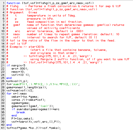
Use of the function to correct the results in Ex 7.3 is shown in the session:
How many streams will there be?3
Here are your compounds' formulae and names:
No. Formula Name
  1  CH3OH      methanol
  2  C3H7OH     n-propanol
  3  CH3COCH3   acetone
>> global Amar
>> Amar=[-.0753 .6495 .557];  <-- From eq. 7.49
>> T=343;      <-- Temperature in K
>> P=101.325;  <-- Pressure in kPa
>> zs=[.4 .2 .4];  <-- Feed mol fraction
>> gamf='marg1';  <-- Name of activity coefficient function
>>  [ts,vof]=flshg(T,P,zs,gamf)
ts =
    0.8883    0.6765    0.9385  <-- Fraction of compounds to Top
vof =
    0.8661  <-- Much larger than the value: 0.046 reported for V/F
>> ns(1,:)=zs  Using the mass balance modules to show all flows
ns =
    0.4000    0.2000    0.4000
         0         0         0
         0         0         0
>> sep(ts,1,[2 3])
>> showm(1,2:3,10,5)
Compound     Inlet    |            Outlet
     Stream         1 |         2         3   Total
 methanol     0.40000 |   0.35533   0.04467   0.40000
 n-propanol   0.20000 |   0.13529   0.06471   0.20000
 acetone      0.40000 |   0.37538   0.02462   0.40000
Total         1.00000 |   0.86601   0.13399   1.00000
>> ys=ns(2,:)/sum(ns(2,:));
>> xs=ns(3,:)/sum(ns(3,:));
>> gams=marg1(xs);
>> ks=kval(T,P).*gams;
>> M=[ys;xs;ks;gams]'
M = <- y         x        K        gamma  Compound
    0.4103    0.3334    1.2302    1.0059  methanol
    0.1562    0.4829    0.3234    1.0002  n-propanol
    0.4335    0.1837    2.3633    1.5045  acetone
After correcting the spread sheet program used to generate the results shown in the text, the authors found:
For this mixture at this temperature and pressure, V/F =
0.8639 and the compositions, K values and activity coefficients are
given by:

           yi       xi   Ki      gi
Methanol 0.4107  0.3319 1.2374 1.00642
Propanol 0.1555  0.4824 0.3224 1.00376
Acetone  0.4337  0.1857 2.3362 1.5014
In this example, we wish to flash a liquid at a higher temperature and pressure (373K and 10 atm.) to atmospheric pressure without adding or subtracting heat from the unit. We can anticipate that this will require additional trial and error to find the temperature that will make the process adiabatic. We can use the mass and energy balance modules to find out how much heat would have to be used for a specified temperature. The case examined in Ex 7.3 would produce:
>> [ts,vof]=flshg(T,P,zs,gamf)
ts =
    0.8883    0.6765    0.9385
vof =
    0.8661
>> setne('l',1,373,zs)
>> sepe('v','l',T,T,1,2:3,ts)
ans =
   25.0908   <-- Thus 25 kJ would have to be added to the flash unit
>> T=340;    <-- We will try a lower temperature.
>> [ts,vof]=flshg(T,P,zs,gamf)
ts =
    0.7210    0.3956    0.8268
vof =
    0.6983
>> sepe('v','l',T,T,1,2:3,ts)
ans =
   18.7848   <-- Now we need only 19 kJ, but we need to lower the
>> T=335;         temperature again.
>> [ts,vof]=flshg(T,P,zs,gamf)
??? Error using ==> fzero  <-- Bad news!
The function values at the interval endpoints must differ in sign.

Error in ==> /home/ceng403/matlab/flshg.m
On line 39  ==>    vof=fzero(fx,vofi,erc,[],P1);
This error in fsolve was found to persist at all temperatures below 339K, a long way from the adiabatic conditions we want.
A second non-ideal flash program was then written that avoided the use of fsolve. It used instead the program ssec2 that has been used at Rice for many years.
An examination of the procedure used in both flshg and flshg2 led to the conclusion that both could give problems associated with the trial and error used to find V/F inside a trial and error used to find the liquid composition.
It might be better and more reliable to look for all the variables at once. We can solve for any number of unknowns using the function: fsolve. It requires an auxiliary function to return an error vector of the same dimension as the number of unknowns. We have one plus the number of compounds as our unknowns. Actually we could reduce that by one by making use of the fact that the mol fractions must sum to one, but that does not help very much. Here is the auxiliary function: flshgaux
This function is used in our third non-ideal flash function: flshg3

Here is a session used to compare the three programs and to determine which might a) require more computation in case we need to do this by hand and b) might be more "robust" and able to handle more difficult cases.
How many streams will there be?3
Here are your compounds' formulae and names:
No. Formula Name
  1  CH3OH      methanol
  2  C3H7OH     n-propanol
  3  CH3COCH3   acetone
>> global Amar
>> Amar=[-.0753 .6495 .557];
>> T=343;
>> P=101.325;
>> zs=[.4 .2 .4];
>> gamf='marg1';
>> fl1=flops
fl1 =
        9283
>> [ts,vof]=flshg(T,P,zs,gamf)
ts =
    0.8883    0.6765    0.9385
vof =
    0.8661
>> dfl=flops-fl1
dfl =
        2603  <-- flshg used only 2603 FLOPs
>> fl1=flops
fl1 =
       11887
>> [ts,vof]=flshg2(T,P,zs,gamf)
ts =
    0.8883    0.6764    0.9384
vof =
    0.8660
>>  dfl=flops-fl1
dfl =
        3515  <-- flshg2 used 3515 FLOPs
>> fl1=flops
fl1 =
       15403
>> [ts,vof]=flshg3(T,P,zs,gamf)
ts =
    0.8882    0.6763    0.9386
vof =
    0.8660
>> dfl=flops-fl1
dfl =
        9597  <-- flshg3 used over 9500 FLOPs
For this case where all three programs converge, it would appear that the use of fsolve to find all four unknowns at once costs a lot of computer time. Part of that extra time may be used to satisfy more stringent convergence tests than were used in the other two programs. Look at what happened when we moved to a lower temperature:
>> [ts,vof]=flshg(335,P,zs,gamf)
??? Error using ==> fzero  <-- we get our error in flshg
The function values at the interval endpoints must differ in sign.

Error in ==> /home/ceng403/matlab/flshg.m
On line 39  ==>    vof=fzero(fx,vofi,erc,[],P1);

>> fl1=flops
fl1 =
       25114
>> [ts,vof]=flshg2(335,P,zs,gamf)
*******************************************************
* ssec2 did not converge, xl:   0.99902 xr:         1 *
*******************************************************
ts =
    0.2445    0.0712    0.3483
vof =
    0.2511
>> dfl=flops-fl1
dfl =
        4118  <-- flshg2 takes a few more FLOPs and gives a warning
>> fl1=flops
fl1 =
       29233
>> [ts,vof]=flshg3(335,P,zs,gamf)
ts =
    0.2456    0.0716    0.3488
vof =
    0.2521
>> dfl=flops-fl1
dfl =
        9032  <-- flshg3 takes fewer FLOPs and does not seem to have
                   any problems.
We will next use the third non-ideal flash program to find the adiabatic temperature for the flash. Here is an auxiliary function that gives the heat required for a given assumed temperature:

Here is the final solution of Example 7.4:
>> global flshP flshTf
>> flshP=P
flshP =
  101.3250
>> flshTf=373
flshTf =
   373
>> flshgad(340)
ans =
   18.7851  <-- Too high
>> flshgad(335)
ans =
    3.2788  <-- Still too high
>> flshgad(333)
ans =
   -9.2870  <-- Too low
>> ssec2([333 335],'flshgad(x)')
ans =
  334.3531  <-- Temperature that should be about right.
>> showe(1,2:3,10,5)
             Inlet    |            Outlet
     Stream         1 |         2         3   Total
  Tmp K        373.00 |    334.35    334.35
  State       liquid  |    vapor    liquid
  Entlpy     -245.864 |   -32.298  -213.566  -245.864
Compound    Stream Flows
 methanol     0.40000 |   0.05874   0.34126   0.40000
 n-propanol   0.20000 |   0.00776   0.19224   0.20000
 acetone      0.40000 |   0.08668   0.31332   0.40000
Total         1.00000 |   0.15318   0.84682   1.00000
Let's make a table like the one reported in the Examples:
>> ns  <-- The molar flows are in the matrix ns
ns =
    0.4000    0.2000    0.4000
    0.0587    0.0078    0.0867
    0.3413    0.1922    0.3133
>> ys=ns(2,:)/sum(ns(2,:))
ys =
    0.3834    0.0507    0.5659
>> xs=ns(3,:)/sum(ns(3,:))
xs =
    0.4030    0.2270    0.3700
>> Ks=ys./xs
Ks =
    0.9515    0.2233    1.5294
>> gams=marg1(xs)
gams =
    1.0903    1.0398    1.2859
>> M=[ys;xs;Ks;gams]'
M =    y         x         K       gamma
    0.3834    0.4030    0.9515    1.0903  methanol
    0.0507    0.2270    0.2233    1.0398  n-propanol
    0.5659    0.3700    1.5294    1.2859  acetone
The authors found using their spread sheet programs:
A temperature of 334.58 K with V/F = 0.1782. The results of the
adiabatic flash are given below:

            yi    xi     Ki     gi
Methanol 0.3874 0.4027 0.9621 1.0877
Propanol 0.0526 0.2320 0.2266 1.0510
Acetone  0.5600 0.3653 1.5330 1.2905