TPWS

TPWS

Thermodynamic Properties of Water and Steam

by Howard Chao and Stella Unruh

Creating/Specifying the Unit Set

All of the calculations found with the IAPWS IF-97 may be converted to any unit. However, because the possibilities of different units are endless, only a select few were built into this application. The header file for tpws_SetUnit.m provides all of the necessary information for changing the unit set. The structure for the unit set is shown below.

Code from tpws_SetUnit.m

...

switch unitSet

% IAPWS Standard

case {'IAPWS','iapws'}

tpwsUnits.T = 'K';

tpwsUnits.p = 'MPa';

tpwsUnits.v = 'm3/kg';

tpwsUnits.e = 'kJ/kg';

tpwsUnits.e2 = 'kJ/kg K';

...

Two default unit sets are preprogrammed into the application (IAPWS and English units). However, the user may create additional custom unit sets to use with the code. However, the desired unit set must be specified in Line 39 of tpws.m. By default, all calculations are made using the IAPWS standard units.

Code from tpws.m

...

% Name of desired unit set

unitSet = 'IAPWS';

% Initialize the data structure

tpwsData = tpws_IntData;

...

Additional units may be added to the library by modifying the files tpws_Convu.m and tpws_ConvuStand.m. This process is rather self-explanatory and only requires a minimal amount of programming knowledge.

Acquiring Thermodynamic Properties

Once the unit set has been properly specified, thermodynamic properties of water and steam are only seconds away! The calling syntax for tpws.m is given in the header file (reproduced below).

Code from tpws.m

...

% Syntax: [tpwsData, tpwsData2] = tpws(p,T,dispTable)

% p Pressure [MPa]

% T Temperature [K]

% dispTable Optional Parameter to disable the table

% display of thermodynamic properties. By

% default, the table feature is enabled.

% 0 = Disable table display

% Note: No action necessary to enable

% table display

% -------------------------------------------------------------------------

% Output: tpwsData Data structure for the properties of water

% tpwsData2 Data structure for the vapor phase

% when the water is saturated (otherwise, no

% data is stored in this parameter)

...

For instance, to determine the properties of water at (5 MPa, 500 K), simply enter the following command into the Matlab command window

>> data1 = tpws(5,500);

Thermodynamic Properties of Water and Steam

-----------------------------------------------------------------------

Temperature 500.00000000 K

Pressure 5.00000000 MPa

Specific Volume 0.00119973 m3/kg

Internal Energy 969.98873381 kJ/kg

Enthalpy 975.98739961 kJ/kg

Entropy 2.57650516 kJ/kg K

Isobaric Heat Capacity 4.63842045 kJ/kg K

Isochoric Heat Capacity 3.21984210 kJ/kg K

State Liquid

-----------------------------------------------------------------------

The data values generated by this code are stored in a data structure. The names of each field are shown below. The code below also shows how to access these fields values individually.

>> data1

data1 =

T: 500

p: 5

v: 0.00119973315866

u: 9.699887338129248e+002

s: 2.57650515860174

h: 9.759873996062026e+002

c_p: 4.63842044505813

c_v: 3.21984209760407

state: 'Liquid'

>> data1.v

ans =

0.00119973315866

For instance, to calculate the difference in enthalpy between water at (5 MPa, 500 K) and (5 MPa, 530 K) we would enter the following

>> data2 = tpws(5,530,0);

>> data2.h – data1.h

ans =

1.431806415316273e+002

Notice that by passing an additional parameter through the calling sequence we have effectively disabled the table display (0 = disable). This may be useful in saving computational time if displaying the table becomes unnecessary.

In order to determine the properties of saturated water, we may make use of the functions region4_pcalc.m and region4_Tcalc.m. The following code shows how to find saturated properties at a given temperature.

>> T = 300;

>> tpws(region4_pcalc(T), T);

Thermodynamic Properties of Water and Steam

-----------------------------------------------------------------------

Temperature 300.00000000 300.00000000 K

Pressure 0.00353659 0.00353659 MPa

Specific Volume 0.00100350 39.08205832 m3/kg

Internal Energy 112.57144185 2411.67581460 kJ/kg

Enthalpy 112.57499081 2549.89300831 kJ/kg

Entropy 0.39312360 8.51753669 kJ/kg K

Isobaric Heat Capacity 4.18137309 1.91393268 kJ/kg K

Isochoric Heat Capacity 4.13100779 1.44209965 kJ/kg K

State Liquid Vapor

-----------------------------------------------------------------------

Likewise, to find saturated water properties at a given pressure use the following sequence.

>> p = 5;

>> tpws(p,region4_Tcalc(p));

Thermodynamic Properties of Water and Steam

-----------------------------------------------------------------------

Temperature 537.09287119 537.09287119 K

Pressure 5.00000000 5.00000000 MPa

Specific Volume 0.00128641 0.03944627 m3/kg

Internal Energy 1148.07001428 2596.99571006 kJ/kg

Enthalpy 1154.50204233 2794.22706605 kJ/kg

Entropy 2.92074596 5.97370405 kJ/kg K

Isobaric Heat Capacity 5.03218240 4.43783773 kJ/kg K

Isochoric Heat Capacity 3.11517459 2.59046427 kJ/kg K

State Liquid Vapor

-----------------------------------------------------------------------

However, when using these commands you MUST be operating under the default IAPWS units (MPa and K).

When performing further calculations involving saturated properties, be sure to pass two data structures to tpws.m because there are two sets of computed thermodynamic data!

>> [liquid, vapor] = tpws(region4_pcalc(373.15), 373.15);

Thermodynamic Properties of Water and Steam

-----------------------------------------------------------------------

Temperature 373.15000000 373.15000000 K

Pressure 0.10141798 0.10141798 MPa

Specific Volume 0.00104346 1.67186060 m3/kg

Internal Energy 418.99332986 2506.01530769 kJ/kg

Enthalpy 419.09915500 2675.57202922 kJ/kg

Entropy 1.30701433 7.35407705 kJ/kg K

Isobaric Heat Capacity 4.21664512 2.07749187 kJ/kg K

Isochoric Heat Capacity 3.76770022 1.55369870 kJ/kg K

State Liquid Vapor

-----------------------------------------------------------------------

Thus, the enthalpy of vaporization at 373.15 K (100°C) may be easily calculated using the following command.

>> vapor.h - liquid.h

ans =

2.256472874223131e+003

Slightly Advanced Topics

Because all of the calculated data may be accessed individually and stored into an array, thermodynamic plots become incredibly easy to construct. For example, the following code will plot the isobaric heat capacity as a function of temperature at constant pressure under the conditions

300 K ≤ T ≤ 1000 K p = 10 MPa.

clear

% Array index counters

k = 1;

j = 1;

% Starting conditions

p = 10; % MPa

T = 300; % K

while (T < 1000)

% Acquire Data using tpws (disable table display)

tpwsData = tpws(p,T,0);

% Store the computed data into proper arrays

switch tpwsData.state

case {'Liquid'}

TdataL(k) = T;

cpdataL(k) = tpwsData.c_p;

k = k + 1;

otherwise

TdataV(j) = T;

cpdataV(j) = tpwsData.c_p;

j = j + 1;

end

% Increment the temperature

T = T + 8;

end

% Plot results

plot(TdataL, cpdataL, '-b.', TdataV, cpdataV, '-r.');

xlabel('T [K]');

ylabel('C_P [kJ/kg K]');

grid on;

A similar plot was obtained from NIST using the same conditions.

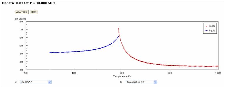
From visual inspection the results from both sources are equivalent! This example illustrates one of the many powerful capabilities of tpws.m.