We notice that an object given a certain distance away from the camera exhibits a disparity in location in the left and right images. Specifically, there is a certain distance for which an object will appear to be at the exact same location in both left and right images. Any object closer will exhibit a positive disparty, for which the right image will show the object to the left of the same image in the left image. Any object further will exhibit a negative disparty, for which the right image will show the object to the right of the same image in the left image. There is a direct correlation between the disparty and the actual distance of the object from the camera.

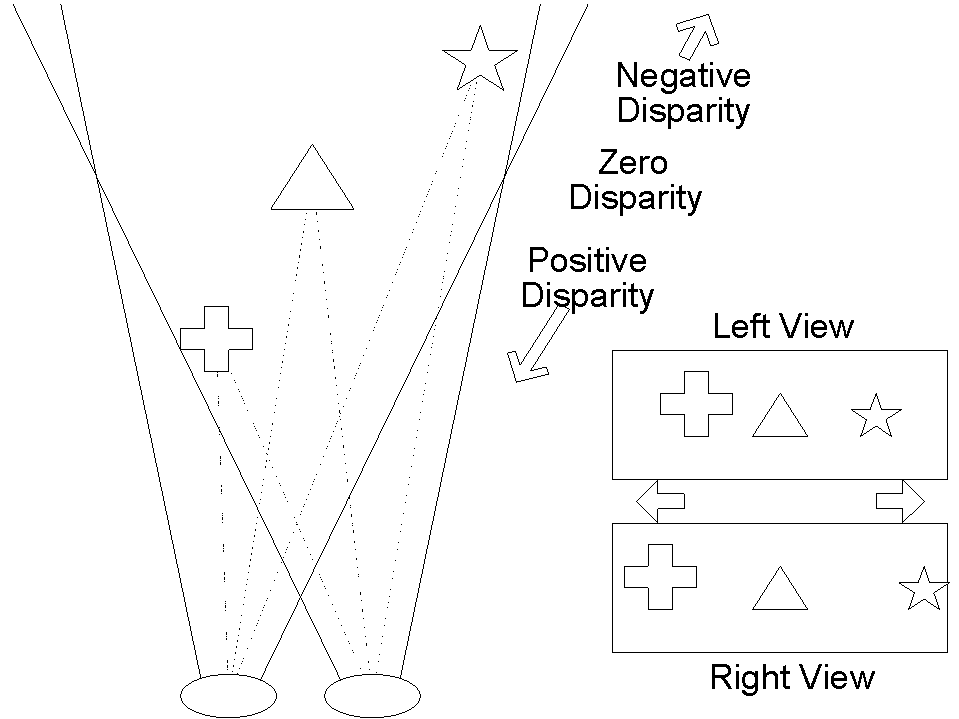
We find this disparity by observing the normalized cross correlation between the left and right images. Different similarity measures have been used in the literature, but it has been shown that the zero mean normalized cross correlation and the zero mean sum of squared differences tend to get better results. This estimate is independent of the differences un brightness and contrast due to the normalization.

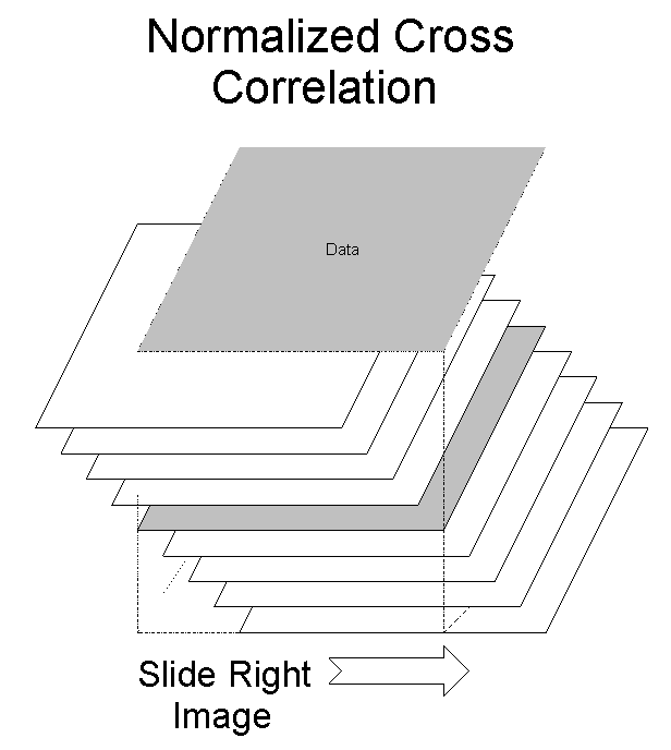
The normalized cross correlation of two windows can be written as follows (with f and g being the intensity values of M x N images at a given position). The variable d refers to a disparity between the two images. In our case, the correlation is performed along the epipolar line. If for any point in the left image, the search window is assumed to be within d = [-w, w] in the right image.

where

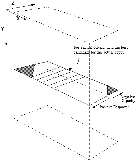
The output of the cross-correlation is a 3D matrix. This diagram shows it's configuration:

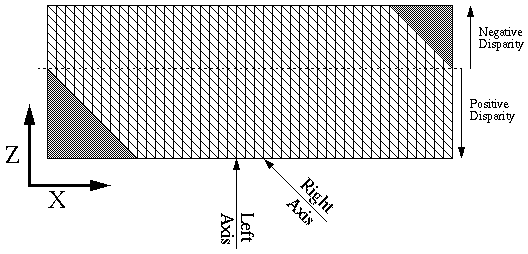
This next diagram is a detail of the cross-section in the matrix. Notice that the left image has a depth axis that lines up with the Z axis and the right image has a depth axis that is along the diagonals. This is because the cross-correlation kept the left image stationary, while the right image moved. It is important to keep in mind that neither the left or right correlation is more important than the other.

The second stage is to extract the correct depth from the correlation matrix. We will have a depth corresponding to every pixel in the image so for each (i, j) point, we get a depth column. This vector contains correlation coefficients and we want the depth of the best match. With a simple case, we simply take the location of the maximum value in the vector. Here is a more complicated/reliable method:

Find each relative peak has a value greater than or equal to its 4 connected neighbors in the uncompressed correlation cube. If we apply multiscaling to the image, we can greatly improve our ability to find the actual disparity, considering a number of low pass images and redefining a peak as having a value greater than or equal to one half the value of the strongest peak along each viewing direction. This basically limits the search space by removing any peaks that are relatively weak. We have arbitrarily chosen to define one half the value of the strongest peak.