The Haar wavelet transform is based on sums and differences where you take the sum and difference of every pair of pixels. By doing this for every row and every column and putting the sums in the left or upper part and the differences in the right or the lower part of the matrix, we obtain a matrix with large values in the upper left quarter and smaller values in the remaining three quarters of the matrix. Iterating this process several times the result will be a matrix with the energy packed in the upper left corner of the matrix. From the resulting matrix it is easy to recover the original data.
To use the packing property of the Haar transform, we wanted to use a bit allocation pattern where L-shaped areas have a certain number of bits/pixel. To see the importance of selecting the bit allocation pattern we tried several patterns and compared the mean-squared-error for different numbers of bits/pixel.
To sumarize what we did, we transformed our images using the Haar wavelet transform and quantized it using different bit allocation patterns. Finally we saved our image as a file and compressed it using the unix function gzip.
Background on Transform Coding
The general idea behind transform coding is to pack the energy of an image into fewer pixels. In the transform domain the pixels with large values are represented with many bits and the ones with small values with fewer bits. Overall the result will be an image with a lower bit/pixel average. It is desired to find the combination of transform and quantizer that achieves the lowest average mean squared error.
To receive good results we desire a transform with the following properties:
- Fast to compute.
- Decorrelated transform coefficients to remove redundancies.
- Pack energy into only a few transform coefficients.
- Preserve energy.
There are several different transforms that could be interesting for transform coding, for example the DFT, Cosine, Sine, Hadamard, Haar, Slant and the Karhunen-Loeve transform. The Karhunen-Loeve transform is optimal in many ways but may have some drawbacks regarding implementation.
After selecting a transform it is time to design a quantizer which uses the energy packing property of the transform. The result will be a pattern where areas of pixels have different number of bits, ranging from 0 to 8. For each number of bits it is necessary to have a specially designed quantizer. However, since it is not necessary to process the pixels with 0 bits designated, only 8 quantizers are required.
When the transformed image is quantized the only steps remaining are coding and storing or transmission.
To summarize the steps involved in transform coding are:
- Transformation
- Determination of bit allocation
- Quantization
- Coding
Implementation
A group of Matlab m-files implement our Haar wavelet transform, quantization, file writing, file reading, dequantization, and inverse wavelet transform.
hwt.m - implementation of the Haar wavelet transform. Takes as input an matrix (image) and the number of iterations of the wavelet transform to perform. Outputs a new matrix, which is the wavelet transform of the original image.
compress.m - writes the compressed information of the wavelet transformed image to a file. Requires three inputs: the wavelet transform to be quantized, a "quantization vector", and the filename to write to. The "quantization vector" is vector of length n+2, where n is the number of iterations used in creating the wavelet transform. The first value in the vector is n, the rest of the values are a "quantization map", which tells the number of bits to quantize each region with.
quantize.m - Quantizes the matrix given in the input to the given number of bits, using the minimum, maximum, and mean of the area to achieve a good quantization scale. The area around the mean is extra-wide, to achieve a better quantization, since it is assumed that many pixels will be near the mean, and should be rounded towards the mean instead of (possibly) away from it.
dequantize.m, decompress.m, ihwt.m - these are the inverses of the above functions.
(note: after our compression scheme was used, further compression was achieved by using gzip, as per class instruction. This, on average, reduced image size by a ratio of 1.5:1)
Results
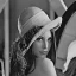
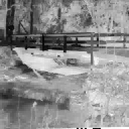
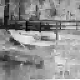
Three images were used test our image compression scheme. The first, of course, was the gorgeous Lenna, whose beautiful face has graced the pages of many signal processing books, papers, and projects. The second and third were the bridge and urban pictures available in the 539 directory. Calculations of PSNR were performed, and plotted against the bits-per pixel. Because we were actually able to produce images of lenna, we performed more tests with lenna than the other two images.
Numerical data of image compression follows. However, as they say, the proof is in the pudding, and our image quality speaks for the viability of our compression:
 |
 |
| 8 bit per pixel Lenna (same size as original, but processed through algorithmn) | 1 bit per pixel Lenna |
 |
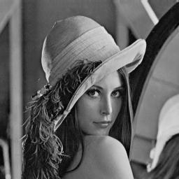 |
| .4 bit per pixel Lenna | Original Lenna |
 |
 |
| .7 BPP Bridge | .4 BPP Bridge |
 |
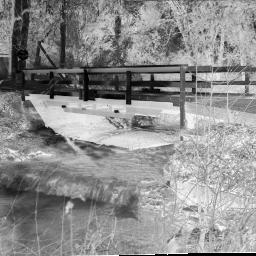 |
| .2 BPP Bridge | Original Bridge |
 |
 |
| .7 BPP Urban | .4 BPP Urban |
 |
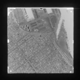 |
| .2 BPP Urban | Original Urban |
|
Bits per pixel (Gzipped) | 5.1 | 1.4 | 1.0 | 0.6 | 0.4 | 0.3 | 0.2 |
|
Mean Square Error (Gzipped) | 1.5 | 112.0 | 114.5 | 138.3 | 276.0 | 296.0 | 316.7 |
| PSNR (Gzipped) | 46.3 | 27.6 | 27.5 | 26.7 | 23.7 | 23.4 | 23.1 |
|
Compression Ratio (Non-Gzipped) | 1.0 | 4.0 | 5.0 | 6.4 | 9.1 | 19.6 | 25.4 |
|
Compression Ratio (Gzipped) | 1.6 | 5.6 | 7.8 | 12.7 | 18.8 | 23.1 | 36.4 |
Plot of PSNR vs. BPP for Lenna
|
Bits per pixel (Gzipped) | .7 | .4 | .2 |
|
Mean Square Error (Gzipped) | 256.9 | 433.9 | 474.8 |
| PSNR (Gzipped) | 24.0 | 21.8 | 21.4 |
|
Compression Ratio (Non-Gzipped) | 6.4 | 15.9 | 25.4 |
|
Compression Ratio (Gzipped) | 10.7 | 18.2 | 36.2 |
|
Bits per pixel (Gzipped) | .5 | .3 | .2 |
|
Mean Square Error (Gzipped) | 65.5 | 141.5 | 158.3 |
| PSNR (Gzipped) | 30 | 26.6 | 26.1 |
|
Compression Ratio (Non-Gzipped) | 6.4 | 15.9 | 25.4 |
|
Compression Ratio (Gzipped) | 14.7 | 23.0 | 50.1 |
(note: for some reason, matlab couldn't save the urban or bridge images with a suitable grayscale colormap, it gave an "index into matrix is negative or zero" eror whenever we tried, thus, they images may look a little odd, but the quality should still be evident.)
Signed:
Ahsan Javed
Adnan Nishat
Erik Sparrman
Michael Sorensen