* What're you guys doing, eh? *
The choice of which transform to use in a transform coder has no clear answer since the performance of a transform compression scheme depends on both the transform and the images being compressed. This project studies the Haar Discrete Wavelet Transform. The Haar DWT is more computationally efficient than the sinusoidal based discrete transforms, but this quality is a tradeoff with decreased energy compaction compared to the DCT.
The Haar transform operates as a square matrix of length N = some integral power of 2. Implementing the discrete Haar transform consists of acting on a matrix row-wise finding the sums and differences of consecutive elements. If the matrix is split in half from top to bottom the sums are stored in one side and the differences in the other. Next operation occurs column-wise, splitting the image in half from left to right, and storing the sums on one half and the differences in the other. The process is repeated on the smaller square, power-of-two matrix resulting in sums of sums. The number of times this process occurs can be thought of as the depth of the transform. In our project, we worked with depth four transforms changing a 256x256 images to a new 256x256 image with a 16x16 purely sums region in the upper-lefthand corner.
Mathematically speaking, this sums and differences approach comes from the Haar functions which are scaled and shifted versions of a single basis function, specifically the odd rectangular pulse pair. Since the Haar transform initiates from a single basis function, the Haar transform identifies edges and lines more directly than sinusoidal based transforms, since the basis function resembles an edge or a line.
Finally, since the vast majority of the energy of an image is stored in the upper-lefthand corner of the transformed matrix, pixel coding can be used to reduce the number of bits necessary to represent the image. Simply use many bits for the high energy region, then fewer and fewer as you progress through the different levels of depth of the transform.
Of course, the proof is in the pudding so the rest of this report will further detail our actions and display the results of our efforts in this area.
* Matlab? What's Matlab? *
In order to implement the image compression algorithm we chose, we divided
the process into various steps:
The first two steps are accomplished using simple loops in
Matlab. Specifically, we wrote two different functions -
rowthing for caluclating
sums and differences of individual rows and colthing for calculating sums and
differences of individual columns.
In order to keep the energy of the image the same, we multiplied each sum
and difference by a factor of 1/sqrt(2). Performing these two operations once
will result in an image that is split into four parts, with the upper left
hand quadrant being the sums of sums region (see Figure 2).
The third step involves repeating the previous two steps until we get down
to a small enough final image. The function squisher accomplishes this task.
This function performs the sums and differences of rows and
columns, in alternating order, until the final sums of sums image is of size
16x16. The resulting image can be seen in the following figure (due to the
normalized display, the various quadrants are not too visible, but contain various edge information):
The next step is quantization. This is performed during the writing to
a binary file (see proceeding discussion of writing to a file); however, we
wrote a distinct quantization function to analyze this step statistically
(MSE and PSNR -- see the Results section), as well as for our own
educational benefit(!). The quantization function, quant, is also called in squisher. Our quantization scheme simply
assigns different numbers of bits to
different regions, using masks (for example, [b16, b32, b64, b128, b256],
where b16 is the quantization level for the upper left 16x16 matrix, b32 is
for the next 32x32 matrix surrounding the first one, etc.). We used a
number of different bit allocation masks (see
next section) in order to determine which scheme is
better.
The quantization function takes in as arguments not only the input
matrix, but also the mask, i.e. the
number of bits to be used to represent each region in the compression
scheme. This allows us to modify and test out difference bit allocation
algorithms easily. The quantized image looks similar to Figure 3, although
depending on the mask used, the level of details may vary.
Once we have generated the compressed matrix, we are ready to transfer it to a
binary file for storage (and, in the process, quantize it). We
use the fwrite Matlab command, specifying the
number of bits with which to quantize. The function bit performs this operation.
Once the file is saved, we can use the file-size information to evaluate
the success of the compression technique. Additionally, a further use of
the lossless gzip command in Unix can show how thoroughly the image could
really be stored. The next section also shows some of these results.
With compression complete, we are ready to decompress and examine the
errors introduced by compression. To reverse our compression scheme, we take the
following steps:
Quantizing the matrix back to its original levels is easy: just quantize
the compressed image back to eight bits, or bitshift 8-(first
quantization level). The function iquant performs this operation.
The inverse sums and differences calculations are made by adding and
subtracting various pairs of numbers in the matrix and dividing by two.
These values are renormalized, and placed in their appropriate positions in
the target matrix. The two functions rowthingi and colthingi accomplishe this task.
These operations are performed first on the columns,
and then on the rows of succeedingly larger sections of the matrix until
the entire 256x256 matrix has been decompressed. This process is done with
the function unsquisher. Once this is
done, we have reconstructed our image. Figure 4 shows the reconstructed
image using the mask [8 6 4 2 0].
* So? Did it work? *
We tested our wavelet transform coder on a few different images to see if
some images would compress better (i.e. with less error) than others. In
addition to the boy.256 image, which is relatively smooth and does not have
too many edges, we also used the following three images:
We ran our coder with various different masks (thus resulting in different
numbers of bits per pixel) on each of these images. For each run, we
determined the mean-square error (MSE) as well as the peak signal-to-noise
ratio (PSNR). The following two graphs show the results of these tests:
As we can see, the boy.256 image seem to perform the best out of the four
while the madrill.256 image seem to perform the worst. We show a nice linear increase in PSNR with additional bits-per-pixel. Note we get a PSNR of greater than 20 for all images even with less than 1 bit per pixel.
In addition to the MES and PSNR results, we also analyzed the results of
the compression (since that is what the assignment is called). For this
analysis, we used the mask [8 6 4 2 0] (the same mask used in the
representative images above) in the coding scheme because it gave us
really good approximations of the original image. For comparison purposes, it is useful
to note that the JPEG compression standard has a compression ratio of 40:1.
(Note: All numbers in units of bytes.)
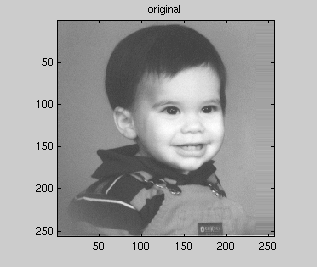
Figure 1 - Original image of
boy.256
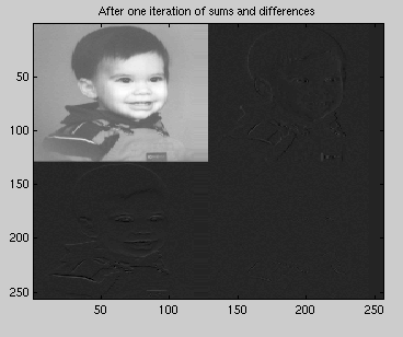
Figure 2 - Sums and differences
after one iteration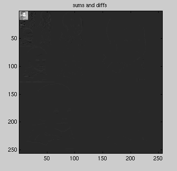
Figure 3 - Final sums and
differences matrix
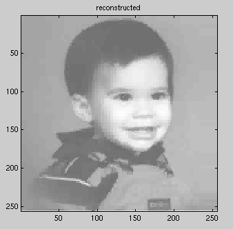
Figure 4 - Reconstructed image
using mask [8 6 4 2 0]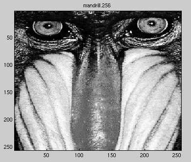
Figure 5 - Image with sharp edges and high contrast
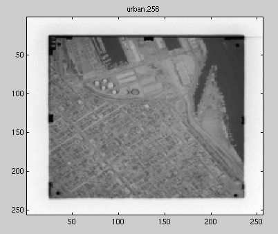
Figure 6 - Blurry satellite image
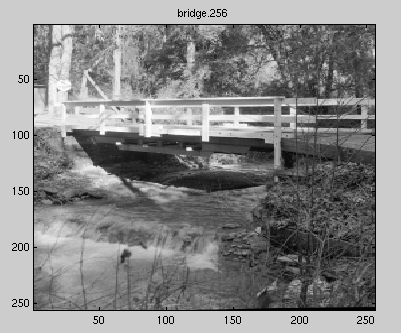
Figure 7 - Image with low contrast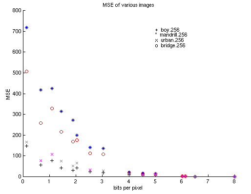
Figure 8 - Mean-square error plot
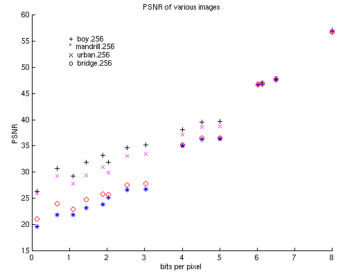
Figure 9 - Peak signal-to-noise ratio
plot