
Craig and Brian stumbled across a web page that gave us a new idea of how to approach this problem. (I think the name of the company is Khoral. The web address for the page is http://www.khoral.com/dipcourse/html/linear/dft-correlation/front-page.html) They recommend a correlation function rather than convolution, and a normalized correlation seems to yield excellant results.
Correlation in 1-D is defined as

Recall that Convolution is just

As was evident with our work last week, the convolution (reverse correlation) by itself does not find the image properly. Maximum points occur where the reels are located, not where the pattern actually is. The resultant "location" matrix depends on the original colors in the image.
In order to solve this problem, Khoral recommends use a slightly different algorithm:
 (i represents a flat color matrix of 1's.)
Rather than create a 2-D correlation function in Matlab, we opted to try the 2-D convolution and see what kind of results we could achieve. If the results were still not up to par, then our next step would be to create a 2-D correlation and run through the complete normalized correlation function.
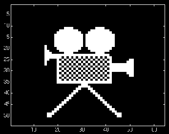
Our template will now be a small bit of the checkerboard pattern.
>> chkboard = movie(25:29,25:29);
>> colormap(gray(max(max(chkboard))));
>> image(chkboard)
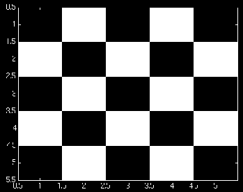
Before we can go on, we will adjust both pictures. Matlab creates the image
as a matrix of ones and twos. In order to get a cleaner picture out, we
change this to a matrix of zeros and ones.
>> movie = movie - 1;
>> chkboard = chkboard - 1;
How effective is the straight 2-D convolution?
>> TwoDConv = conv2(movie,chkboard);
>> colormap(gray(max(max(TwoDConv))));
>> image(TwoDConv)
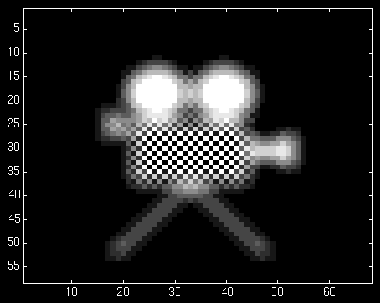
As you can tell, it does a decent job of finding the image, but it also finds a lot of other things! :-)
We now proceed with the normalized correlation procedure. That last step
generated the numerator. Now let's generate the denominator.

>> moviesqr = movie .^2;
>> flat = ones(size(chkboard));
>> norml = conv2(moviesqr,flat);
>> rtnorml = norml .^ 0.5;
>> colormap(gray(max(max(rtnorml))));
>> image(rtnorml);
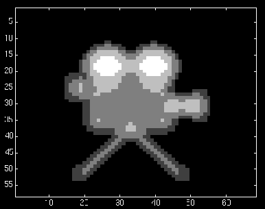
We notice that rtnorml contains several zeros, and since division by zero
is not a good thing, we add a small factor to the denominator and use this
new value in our calculations.
>> rtnorml = rtnorml + .1;
>> cnvnorm = TwoDConv ./ rtnorml;
>> colormap(gray(max(max(cnvnorm))));
>> image(cnvnorm);
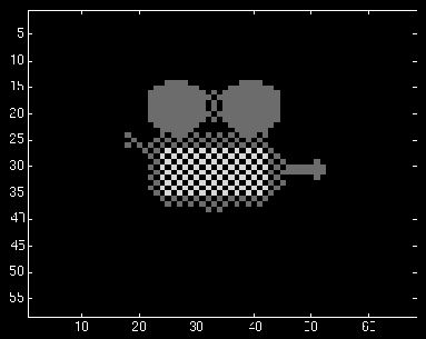
This is pretty good! But, we want to isolate the exact image. At this point
this is just a matter of separating "true" image from "extra." This is just
thresholding.
>> cnvnorm = floor((cnvnorm ./ max(max(cnvnorm))) + 1);
>> colormap(gray(2));
>> image(cnvnorm);
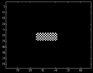
Woo hoo! We found it. Each white pixel represents a place where you can place the template and match it exactly. That's why this final image is a little
smaller than the actual template in the image.

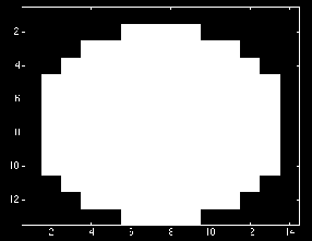
This time, we are trying to find a movie reel. We need the template for it.
>> reel=movie(10:22,18:31);
>> colormap(gray(max(max(reel))));
>> image(reel)
Again, we have to modify our information.
>> movie = movie - 1;
>> reel = reel - 1;
We need the regular 2-D convolution for the numerator of our normalized
correlation function.
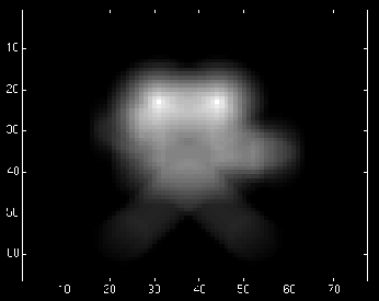
>> TwoDConv = conv2(movie,reel);
>> colormap(gray(max(max(TwoDConv))));
>> image(TwoDConv);
And then we need the denominator.
>> moviesqr = movie .^ 2;
>> flat = ones(size(reel));
>> norml = conv2(moviesqr,flat);
>> rtnorml = norml .^ 0.5;
>> colormap(gray(max(max(rtnorml))));
>> image(rtnorml);
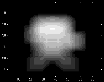
We get rid of the problem with zero division.
>> rtnorml = rtnorml + .1;
>> cnvnorm = TwoDConv ./ rtnorml;
>> colormap(gray(max(max(cnvnorm))));
>> image(cnvnorm);
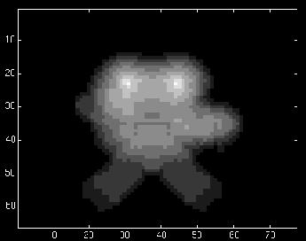
And now we clean up our final image with thresholding. The "floor" function wipes out everything in this case, so we modify our methodology for isolating maximum points.
>> [a,b]=size(cnvnorm);
>> most=max(max(max(cnvnorm)));
>> for rows=1:a
for cols=1:b
if (cnvnorm(rows,cols)<(most-1)) cnvnorm(rows,cols)=0;
end
end
end
>> colormap(gray(2));
>> image(cnvnorm);
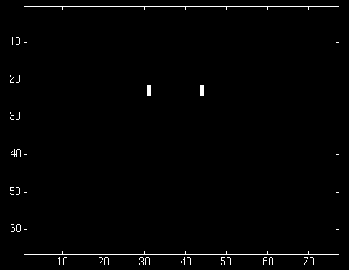
Well, there we have it, folks. Looks like the DSP Pictomaniacs have done a pretty good job so far!