In our modeling of this system we were unable
to do the process in real time. However, the devices with which we
implemented this system are readily available. Thus it can easily be imagined
that the same technology could be combined and implemented in a way that
would actualize this system.
The block diagram of our system
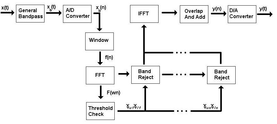
General Bandpass
After some analysis of speech signals, we have determined
a very safe bandwidth for speech that will cut out all frequencies that never
occur in the signal. This band pass goes from 20 Hz (the limit of hearing)
to 10kHz (well above any s-type consonant sounds).
Although this project is for a digital signal processing class,
this portion of our system would probably be best implemented with an analog
bandpass before the signal is converted into a digital signal. Thus
the A/D converter does not need to sample as fast because speech does not
contain these higher frequencies.
A/D Converter
For this experiment we recorded an analog speech signal as well
as a feedback signal with a Sony “Portable MiniDisc Recorder” in conjunction
with a Sony “ECM-MS907 Electret Condenser Microphone”. The A/D converter
in the minidisk player was set to sample a stereo input at 22.050 kHz. The
mic was set to a 90 degree hypercardioid sensitivity shape.
ECM-MS907 SPECIFICATIONS
· Type Mid-Side Stereo; Electret
Condenser Microphone
· Directivity Uni-Directional (stereo);
Directive angle 90 or 120° (switchable)
· Effective Output Level -56 dBm
±4dB (0dB=1mW/Pa, 1kHz)
· Output Impedance 1 kohms ±20%,
unbalanced
· Frequency Response 100 - 15,000Hz
· Maximum Sound Pressure Level
Input more than 110dB SPL
The following filters, computations and algorithms
are all implemented in the software program Matlab 6.1.
Windowing
This is the first step of the analysis and filtering of
the signal. The processor uses a technique called windowing that basically
cuts the signal into smaller pieces so that it can process the speech as
a finite length signal.
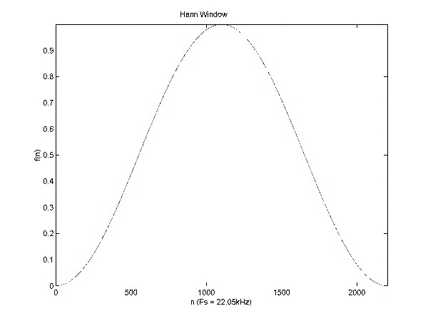
For our particular process we will be using a Hann window.
This window of length n is described by the equation
w[ k + 1 ] = 0.5( 1- cos(2*pi*k/(n-1)) where k
= 0, 1, … n-1
else w[n] = 0
This window is multiplied in the time domain with the signal
so that the only a piece of the signal comes through in the analysis.
The reason we use a smooth filter like Hann instead of a triangle or square
window is that it causes less distortion in the frequency domain.
Once we have windowed this .1 second portion of the signal we begin analysis
for the feedback filter.
FFT
This yields a discrete signal in frequency domain.
f(n) -> F(wn)
After we have taken the FFT of our signal we scan the
signal for high power portions. We set a threshold depending
on the duration of window and in the case that part of the signal is above
the threshold the program records the lower and upper bounds of the section
of the signal that is above the threshold power. These bounds are recoded
for each frequency w that is above the threshold. The bounds are
then input into the band reject portion of the filter.
Band Reject at w
The band reject filter is the key to this suppression
system. The way it works is that it receives threshold boundaries
from the threshold check portion of the system. Then it uses those
boundaries to compute an H(z) which will then be multiplied by the signal
to yield the filtered signal.
F(z) * H(z) = Y(z)
In this case the band reject filter is found using
the following function.
H(z) = z^ –2 – (2ka z^ –1 /
(k+1)) + ((k–1) / ( k+1))
z^ –2(k–1) / ( k+1) – (2a z^ –1 / (k+1)) + 1
z = (1+jw) / (1–jw)
a = cos(( g u + g l ) / 2) / cos(( g u –
g l ) / 2)
k = tan(( g u – g l ) / 2) tan( b / 2)
b = cut-off frequency of model lowpass
filter
g u , g l = desired upper and lower
characteristic frequencies of new filter
IFFT
Once the feedback signals have all been filtered
we implement an Inverse Fast Fourier Transform to return our signal to the
time domain. F(wn) -> f(n)
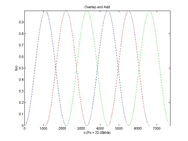
Overlap and Add
This portion takes each of the filtered windows
and adds them back together as seen in the “overlap and add figure”.
This will reproduce our original signal.
D/A Converter
This is simply the internal D/A converter within
the PC. It takes the Matlab vector and turns it back into an analog
signal that is output through the speakers on the PC.