Robot Control

	Feedback Control
	Open-Loop Control
	Feed-Forward Control
	Summary

Sensor Calibration

Manual Sensor Calibration

Dealing with Changing Environmental Conditions

	Light Sensors
	Motor Force Sensing

Using Persistent Global Variables

Robot Control

Sensor Unreliability

Task-Oriented Control

	Exit Conditions
	Timeouts
	Monitoring State Transitions inside a Feedback Loop

Coordination of Tasks

	Task Sequencing
	Concurrent and Non-Competing Tasks
	Concurrent and Competing Tasks
	Robot Metacognition
	Control of an ELEC 201 Robot

Robot Control

The most common kind of robot failure is not mechanical or electronic failure but rather failure of the software that controls the robot. For example, if a robot were to run into a wall, and its front touch sensor did not trigger, the robot would become stuck (unless the robot is a tank), trying to drive through the wall. This robot is not physically stuck, but it is "mentally stuck": its control program does not account for this situation and does not provide a way for the robot to get free. Many robots fail in this way. This chapter will discuss some of the problems typically encountered when using robot sensors, and present a framework for thinking about control that may assist in preventing control failure of ELEC 201 robots.

A few words of advice: most people severely underestimate the amount of time that is necessary to write control software. A program can be hacked together in a couple nights, but if a robot is to be able to deal with a spectrum of situations in a capable way, more work will be required.

Also, it is very difficult to be developing final software while still making hardware changes. Any hardware change will necessitate software changes. Some of these changes may be obvious but others will not. The message is to finalize mechanical and sensor design early enough to develop software based upon a stable hardware platform.

Basic Control Methods

Feedback Control

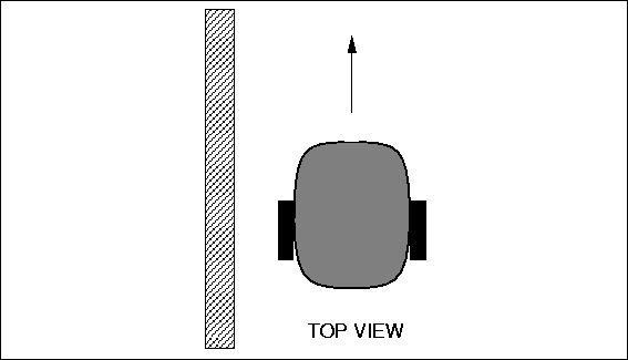
**Figure 11.1:** Driving along a Wall Edge
$\begin{figure} \fbox {\centerline{\psfig{figure=control/edge.PS}}}\end{figure}$

Suppose the robot should be programmed to drive with its left side near a wall, following the wall edge (see Figure 11.1). Several options exist to accomplish this task:

One solution is to orient the robot exactly parallel to the wall, then drive it straight ahead. However, this simple solution has two problems: if the robot is not initially oriented properly, it will fail. Also, unless the robot were extremely proficient at driving straight, it will eventually veer from its path and drive either into the wall or into the game board.

The common and effective solution is to build a negative feedback loop. With continuous monitoring and correction, a goal state (in this case, maintaining a constant distance from a wall) can be achieved.

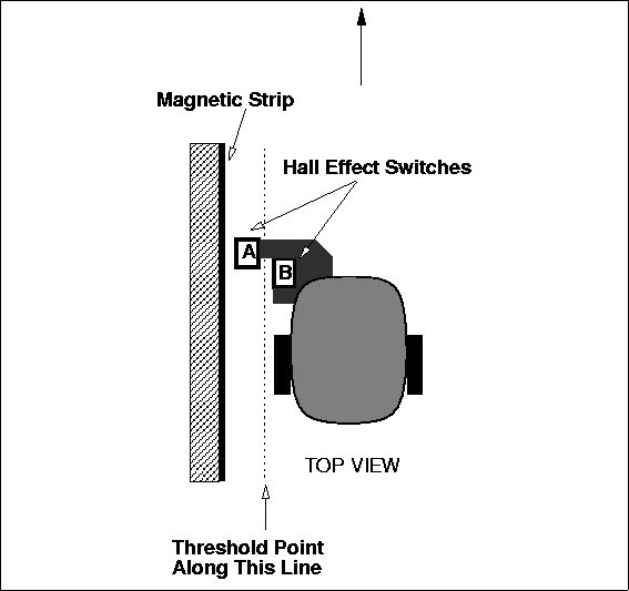
**Figure 11.2:** Using Two Hall Effect Sensors to Follow Wall
$\begin{figure} \fbox {\centerline{\psfig{figure=control/ABedge.PS}}}\end{figure}$

Several of the sensors provided in the ELEC 201 kit can be used to control the distance between the robot and the wall. For example, two Hall effect sensors could be mounted to the robot as shown in Figure 11.2. In this example the wall contains a magnetic strip (as is sometimes the case on the ELEC 201 game board). The two magnetic sensors are mounted on the robot as shown. Since the A sensor is closer to the wall, it will trigger first as the robot moves toward the wall, followed by B if the robot continues to move toward the wall. 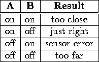As the robot moves away from the wall, B will release first, followed by A if the robot continues to move away from the wall. A decision process making use of this information is depicted in Figure 11.3.

**Figure 11.3:** Control Process With Two Hall Effect Sensors
$\begin{figure} \begin{center} \begin{tabular} {\vert c\vert c\vert c\vert}\hline... ...or\\ \hline off & off & too far \\ \hline\end{tabular}\end{center}\end{figure}$

Notice that the situation with A off and B on is indicative of some failure of the sensor or its mounting.

**Figure 11.4:** Using a Proximity Sensor to Measure Distance to a Wall
$\begin{figure} \fbox {\centerline{\psfig{figure=control/proxwall.ps}}}\end{figure}$

Other sensors provided in the ELEC 201 kit can be used to measure the distance between the robot and the wall (see Figure 11.4). For example, a magnetic field intensity sensor can be used if the wall contains a magnetic strip. In this case the magnetic field sensor would produce a higher value as the robot got closer to the wall. A light source/photocell pair could also be used. In this case the light source (shielded from stray light, perhaps by a cardboard tube) would be aimed at the wall, and the photocell (also shielded from stray light) would produce a value proportional to the distance from a reflective wall. A "bend" sensor could also be used, although the ELEC 201 kit does not contain any of these useful sensors. In this case, the shorter the distance, the more the bend sensor is bent (see explanation of bend sensors).

Suppose a function were written using the two Hall effect sensors to discern four states: TOO_CLOSE, TOO_FAR, JUST_RIGHT (from the wall), and SENSOR_ERROR. Here is a possible definition of the function, called wall_distance():


int TOO_CLOSE= -1;
int JUST_RIGHT= 0;
int TOO_FAR= 1;
int SENSOR_ERROR= -99;

int wall_distance()
{

    /* get reading on A & B sensors */
    int A_value= digital(A_SENSOR);
    int B_value= digital(B_SENSOR);

    /* assume "ON" means the sensor reads zero */
    if ((A_value == 0) && (B_value == 0)) return TOO_CLOSE;
    if ((A_value == 0) && (B_value == 1)) return JUST_RIGHT;
    if ((A_value == 1) && (B_value == 0)) return SENSOR_ERROR;
    /* if ((A_value == 1) && (B_value == 1)) */ return TOO_FAR;

}

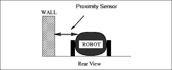
Suppose instead a function were written using a proximity sensor to discern the three states: TOO_CLOSE, TOO_FAR, and JUST_RIGHT. Here is a possible definition of this function, called wall_dist_prox():


int TOO_CLOSE= -1;
int JUST_RIGHT= 0;
int TOO_FAR= 1;
int TOO_CLOSE_THRESHOLD= 50;  /* Embedding threshold constants in this */
int TOO_FAR_THRESHOLD= 150;   /* manner in a real program is not good */
                              /* programming practice.  Instead, they */
                              /* should be placed in a separate file. */

int wall_dist_prox()
{

    /* get reading on proximity sensor */
    int prox_value= analog(PROXIMITY_SENSOR);

    /* assume smaller values mean closer to wall */
    if (prox_value < TOO_CLOSE_THRESHOLD) return TOO_CLOSE;
    if (prox_value > TOO_FAR_THRESHOLD) return TOO_FAR;
    return JUST_RIGHT;

}

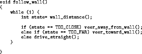
Now, a function to drive the robot making use of the wall_distance() function would create the feedback. In this example, the functions veer_away_from_wall(), veer_toward_wall(), and drive_straight() are used to actually move the robot, as shown in Figure 11.5.

**Figure 11.5:** Wall-Following Function
$\begin{figure} {\small \addtolength {\baselineskip}{-.2\baselineskip} \begin{v... ...AR) veer_toward_wall(); else drive_straight(); } }\end{verbatim}}\end{figure}$

Even if the function to drive the robot straight were not exact (maybe one of the robot's wheels performs better than the other), this function should still accomplish its goal. Suppose the "drive straigh" routine actually veered a bit toward the wall. Then after driving straight for a bit, the "follow wall" routine would notice that the robot was too close to the wall, and execute the "veer away" function.

The actual performance of this algorithm would be influenced by many things, including:

	How sharply the "veer away" and "veer toward" functions made the robot turn.
	The accuracy of the Hall effect switching thresholds, or how well the proximity sensors measured the distance to the wall.
	For proximity sensors, the settings of the `TOO_CLOSE_THRESHOLD` and `TOO_FAR_THRESHOLD` values.
	The rate at which the `follow_wall()` function made corrections to the robot's path.

Still, use of a negative feedback loop ensures basically stable and robust performance, once the parameters are tuned properly.

*The type of feedback just described is called negative feedback because the corrections subtract from the error, making it smaller. With positive feedback, corrections add to the error. Such systems tend to be unstable.

Open-Loop Control

**Figure 11.6:** Negotiating a Corner
$\begin{figure} \fbox {\centerline{\psfig{figure=control/corner.PS}}}\end{figure}$

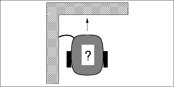
Suppose now the robot has been following the wall, and a touch sensor indicates that it has reached the far edge. The robot needs to turn clockwise ninety degrees to continue following the edge of the wall (see Figure 11.6). How should this be accomplished?

One simple method would be to back up a little and execute a turn command that was timed to accomplish a ninety degree rotation. The following code fragment illustrates this idea:


    ....
    robot_backward(); sleep(.25); /* go backward for 1/4 second */
    robot_spin_clockwise(); sleep(1.5); /* 1.5 sec = 90 degrees */
    ....

This method will work reliably only when the robot is very predictable. For example, one cannot assume that a turn command of 1.5 seconds will always produce a rotation of 90 degrees. Many factors affect the performance of a timed turn, including the battery strength, traction on the surface, and friction in the geartrain.

This method of using a timed turn is called open-loop control (as compared to closed-loop control) because there is no feedback from the commanded action about its effect on the state of the system. If the command is tuned properly and the system is very predictable, open-loop commands can work fine, but generally closed-loop control is necessary for good performance.

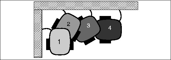
**Figure 11.7:** Negotiating a Corner with Touch Sensor Feedback
$\begin{figure} \fbox {\centerline{\psfig{figure=control/bonk.PS}}}\end{figure}$

How could the corner-negotiation action be made into a closed-loop system? One approach is to have the robot make little turns, drive straight ahead, hit the wall, back up, and repeat (see Figure 11.7), dealing with the corner in a series of little steps.

Feed-Forward Control

There are certain advantages to open-loop control, most notably speed. Clearly a single timed turn would be much faster than a set of small turns, bonks, and back-ups.

One approach when using open-loop control is to use feed-forward control, where the commanded signal is a function of some parameters measured in advance. For the timed turn action, battery strength is probably one of the most significant factors determining the turn's required time. Using feed-forward control, a battery strength measurement would be used to "predict" how much time is needed for the turn. Note that this is still open-loop control -- the feedback is not based on the actual result of a movement command -- but a computation is made to make the control more accurate.

For this example, the battery strength could be measured or estimated based on usage since the last charge.

Summary

For the types of activities commonly performed by ELEC 201 robots, feedback control proves very useful in:

	Wall following. As discussed in this section.
	Line following. Using one or more reflectance sensors aimed at the surface of the ELEC 201 game board.
	Infrared tracking. Homing in on a source of infrared light, using the IR sensors.

Open-loop control should probably be used sparingly and in time-critical applications. Small segments of open-loop actions interspersed between feedback activities should work well.

Feed-forward techniques can enhance the performance of open-loop control when it is used.

Sensor Calibration

Manual Sensor Calibration

The function wall_dist_prox() (one of the examples in Section 11.1.1) used threshold variables (TOO_FAR_THRESHOLD and TOO_CLOSE_THRESHOLD) to interpret the data from the proximity sensor. Depending on the actual reading from the proximity sensors and the settings of these threshold variables, wall_dist_prox() determined if the robot was "too close," "too far," or "just the right" distance from the wall.

Proper calibration of these threshold values is necessary for good robot performance. Often it is convenient to write a routine that allows interactive manipulation of the robot's sensors to determine the proper calibration settings.

For a given proximity sensor, a calibration routine could be included that allows placing the sensor a fixed distance from the wall (the TOO_FAR_THRESHOLD), and then depression of one of the user buttons. The routine would then "capture" the value of the proximity sensor at that point, and use this value as the appropriate threshold. Similarly, sensors could be placed closer to the wall and then captured as the TOO_CLOSE_THRESHOLD value.

Later, the values of these thresholds could be noted when the robot is performing particularly well. These "optimal" settings could be hard-coded as default values. The calibration routine could be kept for use under certain circumstances or if other parameters affecting the robot's performance necessitate readjustment of the calibration settings.

Dealing with Changing Environmental Conditions

Calibration routines are particularly important when environmental conditions cause fluctuations in sensor values. Two sensor types are strongly affected either by external environmental conditions or by the robot's internal state:

Light Sensors.: Heavily affected by room lighting (ambient light), unless extremely well-shielded.
Motor Force Sensing.: Dependent on battery voltage. When battery weakens, force readings increase.

Light Sensors

Any light sensor will operate differently in different amounts of ambient (e.g., room) lighting. For best results when using light sensors, they should be physically shielded from room lighting as much as possible, but this is not usually perfect. Given that room lighting will affect nearly all light sensors to some degree, software should be designed to compensate for room lighting.

When using reflectance-type or break-beam light sensing, controlling the sensor's own illumination source is a good strategy. If a sensor reading is taken with the sensor's own illumination off, the reading due to ambient light is measured. If a reading is then taken with the illumination on, a value combining ambient light plus the sensor's own illumination results. By subtracting these two values, the sensor reading due to its illumination alone can be obtained.

The illumination source control method will not wholly eliminate the influence of ambient light. Further calibration in an actual performance environment will probably be necessary.

Motor Force Sensing

Direct measurement of the battery voltage can be used in a function to compensate for its effect on the motor force readings. However, a simple calibration sequence might suffice.

When the motor is trying to turn but can't, then the motor current increases. The RoboBoard's motor force sensing circuitry allows this current to be measured. Set the wheels of your robot in motion at the speed you intend to drive. Hold the wheel to keep it from turning and take a motor force reading. This reading should be significantly higher than the free spinning motor force. If you want to see if your robot is stuck, take a motor force reading. If you get a value near the stalled reading, your robot is stuck.

This calibration sequence would need to be performed periodically over the life cycle of the motor battery.

Using Persistent Global Variables

A persistent global variable (PGV) is a type of global variable that keeps its state despite pressing reset or turning the robot on and off. PGV'S are ideal for keeping track of calibration settings: after calibrating the robot once, it would not need to be recalibrated until after a new program were downloaded (in general, downloading of code will destroy the previous values of a persistent global, although this can be circumvented as explained in Section 10.7.3).

Using persistent globals requires the creation of an initialization program to allow interactive setting of persistent variable values. A menuing program could be written to use the two user buttons (CHOOSE and ESCAPE) and the RoboKnob variable resistor on the RoboBoard (VR1) to navigate around a series of menus. This program could allow the selection and modification or calibration of any of a number of parameters.

By exiting the initialization program without making any changes, or simply not calling it at all, the robot can operate under the previous settings made to the persistent variables.

The routine could also allow restoration of the default values of all of the globals, returning them to some tested and known-to-work values.

Robot Control

This section presents some ideas about designing software for controlling a robot. The focus is not on low-level coding issues, but on high level concepts about the special situations robots will encounter and ways to address these peculiarities. The approach taken here proposes and examines some control software architectures that will comprise the brains of the robot.

Probably the biggest problem facing a robot is overall system reliability. A robot might face any combination of the following failure modes:

	Mechanical Failures. These might range from temporarily jammed movements to wedged geartrains or a serious mechanical breakdown.
	Electrical Failures. We hope it is safe to assume that the computer itself will not fail but loose connections of motors and sensors are a common problem.
	Sensor Unreliability. Sensors will provide noisy data (data that is sometimes accurate, sometimes not) or data that is simply incorrect (touch sensor fails to be triggered).

The first two of the above problems can be minimized with careful design, but the third category, sensor unreliability, warrants a closer look. Before discussing control ideas further, here is a brief analysis of the sensor problem.

Sensor Unreliability

A variety of problems afflict typical robot sensors:

Spurious Sensor Data.: Most sensors will occasionally generate noise in their output. For example, an infrared sensor might indicate the infrared light is present when actually no light is present. Or, a proximity sensor might give a questionable reading. If the noise is predictable enough, it can be filtered out in software. The noisy IR sensor might not be trusted until it gives some number of consecutive readings in agreement with one another.
However, if the noise problem is very bad, a sensor might be rendered useless -- or worse, dangerous -- if the program running the robot places too much trust in the sensor reading.
Missed Sensor Data.: Affiliated with the problem of noisy data is missed data, where for either electrical or software reasons, a sensor reading is not detected -- a light sensor changes state twice before the software can count it, or a touch sensor jams and fails to trigger.

Corrupted Sensor Data.: As discussed in the previous section on calibration, sensor data can be adversely affected by ambient environmental conditions or battery strength.

To some extent, unruly sensor data can be filtered or otherwise processed "at the source," that is, before higher-level control routines see it. The following example uses the function wall_dist_prox() introduced at the beginning of the chapter:

The wall distance routine gets its data directly from the proximity sensor and then outputs an interpretation of that data. The routine does not process the sensor data in any way -- it does not check for unreasonable data samples, for example. Suppose that the proximity sensor should never report a value above 250, and for some reason, a bogus value is detected. This probably indicates some type of sensor failure, such as an unplugged sensor. It makes sense to intercept this failure locally, where the sensor data is first entered into the software system.

In a similar way, sensor data could be averaged, smoothed, or otherwise processed before interpretation. It is logical to assign individual routines to perform this activity for any sensor that might need to be dealt with in a particular way. Using the multi-tasking capabilities of IC, each sensor or sensor sub-system could be assigned its own C process to perform this activity.

Task-Oriented Control

With so many problems facing a robot, how can it get anything done? Usually, one assumes that these problems do not exist. The insidious part is that most of the time, ignoring the failure modes will work. However, when the failures do occur, they will return to inflict crippling damage to a robot's performance.

Returning again to the wall-following example (as implemented by the function follow_wall() (see Figure 11.5) ), in a worst-case scenario, what could happen while a robot was merrily running along, following a wall? Several possibilities:

1.: The robot could run into an object or a corner, properly triggering a touch sensor.
2.: The robot could run into an object or corner, not triggering a touch sensor.
3.: The robot could wander off away from the wall.
4.: The robot could slam into the wall, get stuck, and conditionally trigger a touch sensor.
5.: The proximity sensor could fall off its mount, causing a series of incorrect sensor readings.

Ideally, control software should expect occurrences of cases like those numbered #1 through #4 and be able to detect case #5.

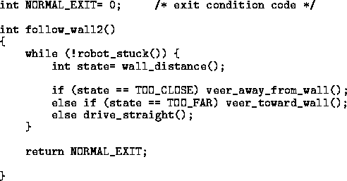
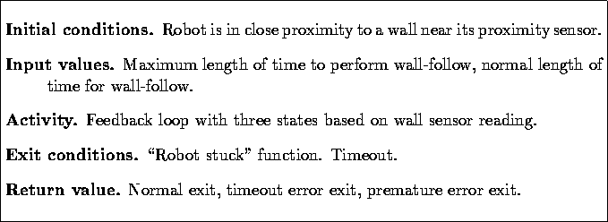
Suppose the wall-following activity is treated as a discrete robot task with initial conditions, an activity to perform (perhaps repetitively), exit conditions, and a return value.

Task Analysis of Simple Wall Follow Function.

$\fbox {\parbox{5.8in}{ \begin{description} \item [Initial conditions.] Robot is ... ...ever exits. \item [Return value.] None, even if it did exit.\end{description}}}$

Exit Conditions

Within this framework, the simple wall-following function could be extended such that it could deal with several of the potential problems it might face while following a wall. Some of these "problems" actually must be dealt with; if a robot doesn't run into an obstacle sooner or later, either something is wrong or the robot is following a very long (circular?) wall.

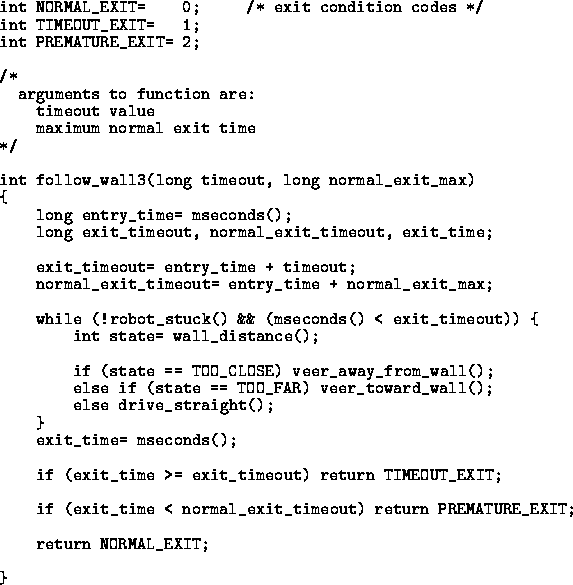
**Figure 11.8:** Wall Following Function with Exit Condition
$\begin{figure} {\small \addtolength {\baselineskip}{-.2\baselineskip} \begin{v... ...; else drive_straight(); } return NORMAL_EXIT; }\end{verbatim}}\end{figure}$

By adding a test for touch sensors inside the loop code of follow_wall(), a function that exits upon detection of a collision can be created. This new function, follow_wall2(), is shown in Figure 11.8. Note the new sensor function robot_stuck(), which is expected to return a boolean true if it believes that the robot is stuck. To double-check that the robot is stuck, the function can get additional data from any of the robot's sensors -- including touch sensors, shaft encoders, and motor force sensors.

Timeouts

Detecting collisions can only be as good as the collision sensors. Since such sensors are not perfect, it may be a good idea to add some kind of timer-based exit condition. This will prevent the case of a robot from getting stuck and not having its touch sensor depressed. Often a robot simply does not "believe" that it is stuck -- its program stays stuck in some loop and does not properly react.

Time-outs can solve this problems and provide other information as well. In a typical application, the maximum time that the robot is allowed to take in performing a particular task would be determined. When the function to perform the task is invoked, it would be given this maximum time. If (continuing the example) the wall-following task failed to exit before the time limit had expired, the timeout would trigger and cause the function to exit (with an appropriate error return value).

Additionally, the timing information could be used to verify that the task had exited normally. If a robot is supposed to take six seconds to get from the start of the wall-follow to another wall and in one instance takes only three seconds, then probably an obstacle caused the premature exit.

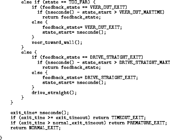
**Figure 11.9:** Wall Following Function with Exit and Timeout Conditions
$\begin{figure} {\small \addtolength {\baselineskip}{-.2\baselineskip} \begin{v... ...eout) return PREMATURE_EXIT; return NORMAL_EXIT; }\end{verbatim}}\end{figure}$

Figure 11.9 lists the third wall-following function, with added timeout capability. Note that the timing variables are defined in long integers (timing units in milliseconds). Floating point variables could also have been used (with the more intuitive units of seconds), but long integers are much more efficient.

A task analysis of the follow_wall3() function shows a much better set of specifications, as shown in Figure 11.10.

**Figure 11.10:** Task Analysis of Wall Follow Function with Sensing and Timeout
$\begin{figure} \fbox {\parbox{5.8in}{ \begin{description} \item [Initial conditi... ...l exit, timeout error exit, premature error exit.\end{description}}}\end{figure}$

Monitoring State Transitions inside a Feedback Loop

The third version of the wall-following function ensures that the robot will not wedge and get stuck forever. However, going a step further, a program can be written to detect failure situations in advance of the overall task timeout.

The key is in the guts of the feedback loop, associated with the functions veer_away_from_wall(), veer_toward_wall(), and drive_straight(). When the robot is following a wall normally, these functions should alternate control, each being operative for only a short period of time. Said another way: the robot will not simply drive straight for a long time, it will veer into the wall for a bit, veer away from the wall for a bit, drive straight for a bit, etc. Conversely, if the robot wandered away from the wall, then the veer_toward_wall() output would be continuously asserted.

Monitoring for normal exchange of control among these feedback outputs allows detection of the feedback loop's normal operation. Conversely, by looking for abnormal exchange of control -- in particular, one output being asserted for too long a period of time -- failure conditions can be detected.

**Figure 11.11:** Wall Following Function with Exit, Timeout, and Feedback Monitoring Conditions, Page 1
$\begin{figure} {\small \addtolength {\baselineskip}{-.2\baselineskip} \begin{v... ...nerate movement command */ veer_away_from_wall(); }\end{verbatim}}\end{figure}$

**Figure 11.12:** Wall Following Function with Exit, Timeout, and Feedback Monitoring Conditions, Page 2
$\begin{figure} {\small \addtolength {\baselineskip}{-.2\baselineskip} \begin{v... ...meout) return PREMATURE_EXIT; return NORMAL_EXIT; }\end{verbatim}}\end{figure}$

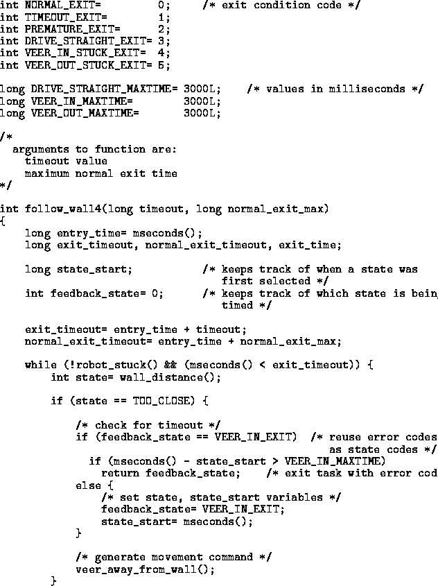
The code to implement this idea works as follows: each time a new feedback output is selected, a timer is reset. The timer measures time spent in consecutive selections of the feedback output. If the same feedback output is selected repeatedly for too long a period of time, an exit error condition is generated.

Several constants are used to adjust the parameters of the timeout: DRIVE_STRAIGHT_MAXTIME, VEER_IN_MAXTIME, and VEER_OUT_MAXTIME. Three new exit error conditions are used to report which part of the feedback loop failed. The final program, follow_wall4(), is shown in Figures 11.11 and 11.12.

One potential problem: It is conceivable that for some duration of time that it would be correct for the loop to stay in one state for an unusually long period of time, in which case this method would incorrectly cause a premature exit. In the wall-following example, if the robot were perhaps to drive very straight and were oriented exactly parallel to the wall, it would be proper to stay in the "drive straight" state for a long while.

Increasing the timeout values of the constants would minimize the potential of this problem -- at the expense of the method's effectiveness. It is probably best to deal with these circumstances on a case-by-case basis. One possibility is to deliberately handicap the feedback control so that it oscillates a bit; clearly this has disadvantages too.

Coordination of Tasks

The robot task model just presented should prove a useful way to make a robot's behavior more reliable. But further questions come up: How should the selection and execution of different tasks be done?

This question is often asked by contemporary robot researchers. In addition to a variety of ways of thinking about robot tasks, there are many different approaches to organizing the higher-level control of mobile robots.

Unlike robots used more generally in research, ELEC 201 robots have special requirements: these robots must be fast; many research robots can sit and compute for a while. ELEC 201 robots must be reliable, whereas for other demonstrations, a robot might be videotaped until it does what the programmers want it to. ELEC 201 robots have only a few chances to perform correctly for the competition; in some research experiments, software robots are "evolved" through many generations until they behave appropriately.

Still, some of the ideas from the research field may be helpful. To extend from the task model developed in this chapter, here are several different approaches that could be used to coordinate and control task execution.

Task Sequencing

In this model, only one task executes at a time. A "task manager" is responsible for selecting tasks based upon a predetermined task sequence, with alternative sequences to deal with exceptional circumstances. This can be visualized as a connected graph of tasks, with the path of traversal determined by the task manager.

A simple example of task sequencing would be a program to make a robot follow the inside wall of a rectangular area. The task manager would alternately invoke "follow wall" and "negotiate corner" tasks, assuming there were no errors.

Concurrent and Non-Competing Tasks

This model builds on the task sequencing model by allowing concurrent execution of tasks that are essentially non-interfering. For example, a task to control a "radar dish" sensor (that locates sources of infrared light) can be operated independently from a task that drives the robot. There may be some communication between the tasks (the radar dish task may wish to know that the robot's base is moving), but there is no direct interference or need for coordination between the tasks.

Concurrent and Competing Tasks

In the most general situation, concurrent tasks might interfere with each other, or compete for resources on the robot (such as control of drive motors or control of an active sensor). In this case, some method, either explicit or implicit, must be devised to resolve resource conflicts.

One method is to provide each task with a priority level; if two or more tasks are competing for the same resource, the task with the highest priority would win. A method for dealing with ties would be needed as well.

Robot Metacognition

A sophisticated task manager might have a separate module that acts as its "overseer." To use Marvin Minsky's idea and terminology from his Society of Mind, the main part of our brains (the "A brain") might be observed by a separate part of the brain (the "B brain").

The B brain, or overseer, checks the A-brain (which is mostly in control) for things like non-productive loops and other wedged conditions. If it detects one of these undesirable states, it makes an intervention that will provoke a different response from the A brain.

Here is an example to bring this metaphor back to our robots. Suppose a task manager (of the sequencer variety) is trying to drive the robot around the inside of a rectangle, as suggested earlier. It is alternating between two tasks: a "follow wall" task and a "negotiate corner" task. But suppose the corner routine is failing, and unbeknownst to the sequencer, the robot is stuck in the same corner.

The robot's "B-brain controller" might notice an especially tight loop between the execution of the two tasks (much the same as the wall-follower would notice trouble in shifting between the feedback outputs). The B-brain would conclude that something had gone wrong, and execute an emergency "get unwedged task.

Control of an ELEC 201 Robot

Most robots have been designed with the "task sequencer" model in mind. Occasionally concurrent, non-competing tasks are employed, but only rarely are concurrent and competing tasks considered.

Rather than advocating a specific method, it is left for the reader to think about these issues and decide what is best for his or her own robot. Some of these methods were developed to make robots more "creature-like," which is not necessarily a desirable characteristic for an ELEC 201 robot. For example, it would not be ideal for a robot to suddenly decide that it did not really want to follow that wall. A task sequencing method, perhaps with a few checks for unproductive loops, should be more than adequate for most robot ELEC 201 designs.