This section of the CENG 403 site presents the modeling of a binary distillation system using Aspen. The system modeled in Aspen may also be investigated using Matlab.

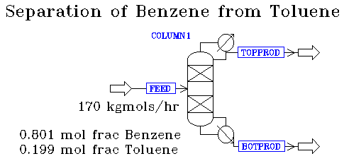
Below is a PFD of the system we wish to model in Aspen.

Since the Matlab distillation modules can only model binary distillation systems, we will continue to use this simplification in Aspen. Keep in mind, however, that Aspen has much more flexibility built into its code, so it is possible to separate streams more complex that a binary stream. For consistency, though, a binary stream will be used in the Aspen model.

The stream we wish to separate is made up of two compounds--benzene and toluene. The mole fraction of each in the feed stream is 0.801 for benzene and 0.199 for toluene. The desired output for this system is 265 lb mol of benzene at a purity of 0.9997; this product will be attained from a feed stream of 170 kgmols/hr.

Aspen allows the user to model distillation columns in several different ways. The easiest model in Aspen is the DSTWU module, which requires fewer operating parameters than any of the other Aspen distillation units.

From the Matlab example, here is a list of constraints that must be met in the separation:

• Feed is 0.801 mol fraction benzene.
• Top product must be 0.9997 mol fraction benzene.
• Process 170 kgmol/hr of feed.
• Produce a bottom product that is 5 mol per cent benzene.
• Feed stream is a saturated liquid.
• Operates at a reflux ratio that is 20% higher than the minimum.
• Operates at a pressure close to atmosphere.

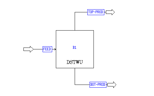
Your working diagram of the Aspen model should look something like this.

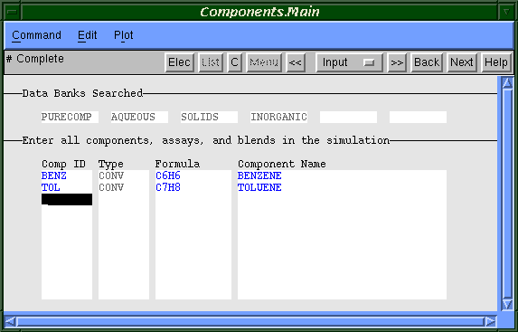
To make this image, you will need one "FEED" arrow, two "PROD" arrows, and one DSTWU icon (found under "Column" in the "Type" menu on the right side of the main Aspen window). Once your flowsheet is complete, click on the "Next" button until the "Setup.Main" window appears. In this window, change "NOMOLEFRAC" to "MOLEFRAC." Then hit "Next." Fill out the Account window appropriately and depress "Next" again. We you get to the "Components.Main" page, fill it in such that it looks like this.

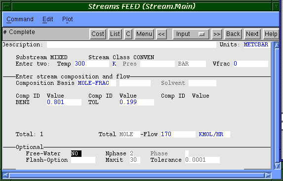
Once you have completed this step, click on "Next." On the "Properties" page that just appeared, type "IDEAL" in the Opsetname box. The Matlab model of this system assumes that the system is ideal, so we will use ideal conditions in Aspen as well. Press the "Next" button until the "Stream.Main" window appears. In this window, we will specify the conditions of the "FEED" stream. When finished, your window should look like this.

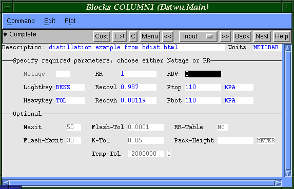
Again, when this is completed, depress the "Next" button. The next window is the "Dstwu.Main" window, which is where you specify the conditions inside the distillation column.

For comparison purposes, we are going to run the model using two different sets of conditions in the column. For the first run, we are arbitrarily going to pick the reflux ratio. After running the simulation, we will be able to determine what the minimum reflux ratio is since Aspen will calculate that for us. In the second run, we will set the reflux ratio such that it is 20% greater than the minimum. We will then compare these results to the Matlab model.

Below is a copy of the window in which you specify the column conditions. Note that the reflux ratio that was chosen is equal to one. We do this because we first want to find out what the minimum reflux ratio is. Thus, complete your window until it looks like the one below.

To determine the minimum reflux ratio, pull up the results window, and click on the ">>" button until you see the following window.

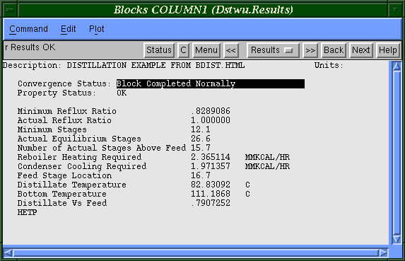
Aspen's minimum reflux ratio is 0.829. This compares favorably with Matlab's answer of 0.821. Since we need the reflux ratio to be 20% higher than this minimum, change the column specifications in Aspen such that the reflux ratio is 1.2*(0.829) or 0.995. Then run the simulation again. Since our original guess of one for the reflux ratio is close to 0.995, the results will not be very different from the first run. Below is a copy of the same results page as above, except the reflux ratio is now 0.995.

Notice that the number of plates in the column is different in the Aspen (27) example than it is in the Matlab example (35). This most likely may be attributed to two reasons. First, the Aspen method uses Winn-Underwood-Gilliland method, which is slightly different from the ideal method using in the Matlab example. Furthermore, keep in mind that the upper half of the McCabe-Thiele diagram for this system is tight. Because of this, slight differences in answers could very well mean a large difference in the number of plates.