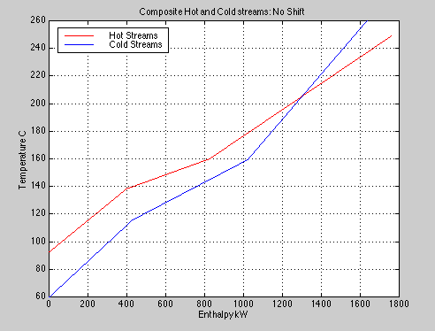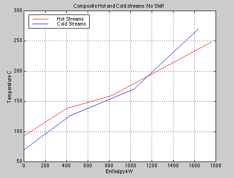
First we will construct composite cold and hot stream data. The following table gives the total value for F*Cp for each temperature interval. For example: C1 is the only cold stream that is heated from 60 to 116, thus the value of F*Cp is 7.62 in that interval.
|
- |
- |
Stream Data |
- |
- |
|
Cold |
Streams |
|
Hot |
Streams |
|
Temp in °C |
F*Cp in kW/°C |
|
Temp in °C |
F*Cp in kW/°C |
|
260 |
- |
|
249 |
- |
|
to |
6.08 |
|
to |
10.55 |
|
160 |
- |
|
160 |
- |
|
to |
13.70 |
|
to |
19.34 |
|
116 |
- |
|
138 |
- |
|
to |
7.62 |
|
to |
8.79 |
|
60 |
- |
|
93 |
- |
In Matlab session:
>> Tcold=[60 116 160 260];
>> FCcold=[7.62 13.7 6.08];
>> Thot=[93 138 160 249];
>> FChot=[8.79 19.34 10.55];
>> help entHC

Uses entHC1 to produce composite curves and plot them with a
horizontal shift
function entHC(Thot,FChot,Tcold,FCcold,Tunit,Hunit)
>> entHC(Thot,FChot,Tcold,FCcold,'C','kW')
That gave us the unshifted composite curves for both the hot and cold streams. Since they cross, it is obvious that we can not construct heat exchangers that will transfer the required heat from the hot streams to the cold ones. Before using a shift to correct for the crossing, we will add a margin of 10C to our system. This can be easily done by adding 10 to Tcold:
If you want to print the current graph, reply: y
Give a new shift or 0 to stop. 0
>> entHC(Thot,FChot,Tcold+10,FCcold,'C','kW')
It is not obvious what shift will be able to prevent the crossing of the two curves, but our later analysis will show that 250.1 kW is required.
If you want to print the current graph, reply: y Give a new shift or 0 to stop. 250.1If you want to print the current graph, reply: y Give a new shift or 0 to stop. 0 >>
Now, we will construct most of the columns in Table 10.7 of BGW. First we need to decide on a minimum temperature difference between hot and cold streams and will use 10C. Next we will establish all temperature intervals where there are different number of streams that are being heated or cooled. In doing this we will shift the cold temperatures up 10C. The columns showing the temperatures for the hot streams have parentheses around them if they came from cold streams with 10 added to them. The cold stream temperatures are also shown in parentheses if they came from hot streams shifted down by 10. We find there are 7 intervals. We will use Matlab to find the available heat from the hot streams in each interval and the heat required to increase the temperatures of the cold streams in the intervals.
Int  Temps       Avail    Reqd      Net        Net      Net
       C           Ht      Ht        Ht     Cascade   Adj. Cas.
    Hot  Cold
   (270)  260                                  0.00   127.68
 7                0.00   127.68   -127.68
    249  (239)                              -127.68     0.00
 6              833.45   480.32    353.13
   (170)  160                                225.45   353.13
 5              105.50   137.00    -31.50
    160  (150)                               193.95   321.63
 4              425.48   301.40    124.08
    138  (128)                               318.03   445.71
 3              105.48   164.40    -58.92
   (126)  116                                259.11   386.79
 2              290.07   251.46     38.61
     93   (83)                               297.72   425.40
 1                0.00   175.26   -175.26
    (70)   60                                122.46   250.14
First, put the cold temperatures at the ends of each interval in the vector Tc:
>> Tc=[60 83 116 128 150 160 239 260]
Tc =
60 83 116 128 150 160 239 260
Next find the temperatur differences in each interval:
>> help diff

DIFF Difference and approximate derivative.
DIFF(X), for a vector X, is [X(2)-X(1) X(3)-X(2) ... X(n)-X(n-1)].
    .......
>> dTc=diff(Tc)
dTc =
23 33 12 22 10 79 21
Next, put in the F*Cp for the total of the cold streams in the vector Fc so we can get the heat required to change the temperatures for the cold streams by a simple multiply. The heat required terms will be put in dHc.
>> Fc=[7.62 7.62 13.70 13.70 13.70 6.08 6.08]
Fc =
7.6200 7.6200 13.7000 13.7000 13.7000 6.0800 6.0800
>> dHc=Fc.*dTc
dHc =
175.2600 251.4600 164.4000 301.4000 137.0000 480.3200 127.6800
Repeat all this for the hot streams.
>> Th=[70 93 126 138 160 170 249 270];
>> dTh=diff(Th)
dTh =
23 33 12 22 10 79 21  <-- These had better be the same as in dTc.
>> Fh=[0 8.79 8.79 19.34 10.55 10.55 0];
>> dHh=dTh.*Fh  <-- Getting the heat available in each interval.
dHh =
0 290.0700 105.4800 425.4800 105.5000 833.4500 0
>> dHnet=dHh-dHc  <-- The net heat is the difference.
dHnet =
-175.2600 38.6100 -58.9200 124.0800 -31.5000 353.1300 -127.6800
>> dHn=dHnet(7:-1:1)  <-- Reversing the listing to make the hottest
dHn =                 intervals be first.
-127.6800 353.1300 -31.5000 124.0800 -58.9200 38.6100 -175.2600
>> dHcas=[0,cumsum(dHn)]  <-- Creating a cascade showing how much heat
dHcas =                    is available above each level.
Columns 1 through 7
0 -127.6800 225.4500 193.9500 318.0300 259.1100 297.7200
Column 8
122.4600
>> dHadj=dHcas-min(dHcas)  <-- Adjusting by adding the minimum amount
dHadj =                     that will make all elements positive.
Columns 1 through 7
127.6800 0 353.1300 321.6300 445.7100 386.7900 425.4000
Column 8
250.1400
Now we can plot the temperatures vs the adjusted heat available vector to create the "Grand Composite Curve" for the streams.
>> plot(dHadj,Th(8:-1:1))
>> grid
>> save BGW4SP1  <-- In case we want to use the data again.
>> title('Grand Composite Curve for 4SP1: dTmin=10C')
>> xlabel('Adjusted Cascaded Heat kW')
>> ylabel('Temp of Hot Stream C')

This curve shows that: