Example 23.5-3: Linear Cascades

>

We saw in example 23.1-2 that the degree of separation possible in a simple binary splitter can be quite limited, and it is therefore often desirable to combine individual splitters in a countercurrent cascade such as that shown in figure 23.5-5. Here the feed to any splitter stage is the sum of the waste stream from the splitter immediately above it and the product from the splitter immediately below.

Product (P)

^

_____ |_____ _ _ _ _ = y stream (gas)

---> | | ---- 1

| | | . . . . . . . = x stream (liquid)

| |__________ | .

| .

| __________ .

| | | .

|__ | | <--- 2

. |__________ | |

. |

. __________ |

. | | |

Feed (F) - -->---> | | ___| 3

| |__________ | .

| .

| __________ .

| | | .

|__ | | <--- 4

. |__________ | |

. |

. __________ |

. | | |

---> | | ___| 5

|__________ |

|

V

Waste (W)

Ø restart;

We can consider the whole system and write a mass balance for the desired product (we would consider the entire system as if it was one splitter).

Ø eq1:= z_F*F = y_P*P + x_W*W; eq2:= F = P + W; equations 23.5-28,29

Let's consider a mass balance over the top portion of the column:

Ø eq3:= y[n]*Up[n] - x[n-1]*Down[n-1] = y_P*P; equation 23.5-30

Ø eq4:= P = Up[n] - Down[n-1]; equation 23.5-31

In these last 2 equations, Up[n] and Down[n-1] are the upflowing and downflowing streams from stages n and n-1, respectively

Ø P:= solve(eq4,P); eq3; substituting the value for P into eq3

Ø eq5:= Downnminus1_Upn = solve(eq3,Down[n-1])/Up[n]; equation 23.5-32

We know, from equation 23.1-19 (Example 23.1-2) that y[n] and x[n] are related by

Ø y[n]:= alpha*x[n]/(1 + (alpha-1)*x[n]);

TOTAL REFLUX

>

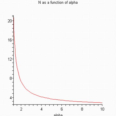
In total reflux, both P and W are equal to 0. This special mode of operation is important since it provides the smallest possible number of stages that can yield the desired output composition.

Ø Up[n]:= Down[n-1]; equation 23.5-34

Ø eq6:=log((y_P/(1-y_P))/(x_W/(1-x_W)))=(N-1)*log(alpha);

> N:= solve(eq6, N): getting the smallest number of stages that can yield the desired output composition

Ø N:= unapply(N,y_P,x_W,alpha);

Ø N(0.9,0.1,2.5); with a product mole fraction of 0.9, a waste mole fraction of 0.1, and a separation factor of 2.5 (we see that it is the same as in BS&L)

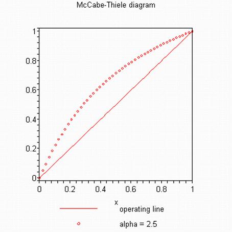
> with(plots):

Warning, the name changecoords has been redefined

> op_line:= plot(x, x=0..1, legend=`operating line`): operation line y[n] = x[n-1]

alpha:= 2.5: value for the separation factor

equil_line:= plot(alpha*x/(1 + (alpha-1)*x), x=0..1, style=point, legend=`alpha = 2.5`): equilibrium line (in the form of eq. 23.5-34)

display({op_line, equil_line}, axes=boxed, title=`McCabe-Thiele diagram`);

> alpha:= 'alpha': y_P:= 0.9: x_W:= 0.1: N:= solve(eq6, N): getting the smallest number of stages that can yield the desired output composition

> N:= unapply(N,alpha): making N a function of alpha

> plot(N(alpha), alpha=1.25..10, title=`N as a function of alpha`);