Continuity Equation

>

restart;

Assumptions:

 1) Assume the flowing fluid will always be nearly pure solvent S.

     Neither A or B will be present in any large quantity.

 2) Diffusion of A in S can be described by the steady-state version of Eq. 19.1-14.

 3) Consider rho*Das = constant

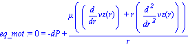
Based on this assumption, the relevant continuity equations and motion equations are those below.

>	eq_mot:=0=-dP+mu*1/r*diff(r*diff(vz(r),r),r);

Determination of Velocity Profile Based on Equation of Continuity

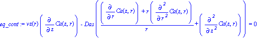
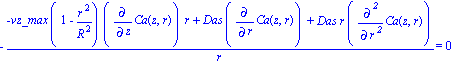
>	eq_cont:=vz(r)*diff(Ca(z,r),z)-Das*(1/r*diff(r*diff(Ca(z,r),r),r)+diff(diff(Ca(z,r),z),z))=0;

Assumptions:

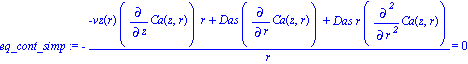
 4) Axial diffusion can be neglected with respect to axial convection.  Therefore, the second derivative term drops.

>	eq_cont_simp:=simplify( lhs(eq_cont)+Das*diff(diff(Ca(z,r),z),z)=rhs(eq_cont) );

Boundary Conditions:

 1) at r=R, vz = 0 (no slip conditions)

 2) at r=0, vz = finite

>	velocity_z(r):=dsolve({eq_mot,vz(R)=0},vz(r));

Since at r=0 (the middle of the pipe), the velocity profile must be finite.  Therefore, _C1 must be 0 so that ln(r) doesn't blow up.

>	velocity_z(r):=1/4*dP*r^2/mu-1/4*(dP*R^2)/mu;

Since dP is defined as P(L)-P(0), but vz_max is defined as (P(0)-P(L))*R^2/(4*mu), there needs to be a sign change here to use the definition of vx_max.

>	vz_corrected2(r):=simplify( velocity_z(r)*(-1) );

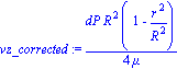
Factoring out a R^2 from the lhs and combining terms, we get the below equation.  The equality of these two equations is also verified.

>	vz_corrected:=dP*R^2/(4*mu)*(1-(r/R)^2);

>	simplify( vz_corrected - vz_corrected2(r) );

Using the given definition of vz_max, we get the final equation for vz(r);

>	dP:=vz_max*4*mu/R^2;

>	vz_corrected;

>	vz(r):=vz_corrected;

>	eq_cont_simp;

Determination of Velocity Profile Based on Momentum Balance

Performing a balance with pressure and shear forces.  As seen before, the velocity vz is only a function of r, not z.

Therefore, the velocity does not change with position horizontally in the tube.

>

restart;

>	Pin:=2*Pi*r*dr*P0;Pout:=2*Pi*r*dr*PL;

>	tau:=r->tau_rz(r)*2*Pi*r*L;

>	tau(r);tau(r+dr);

>	eq_mom:=simplify( limit(( Pin-Pout+tau(r)-tau(r+dr) ) /(2*Pi*L*dr),dr=0 ) );

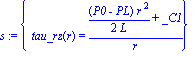
>	s:=dsolve({eq_mom},tau_rz(r));

Boundary Coditions:

 1) at r = 0, tau_rz must be finite

Because of this, we see that a term of _C1/r appears.  This will not give a finite value, and therefore _C1 must be 0.

>	meq:=tau_rz(r)=(1/2*(P0-PL)*r/L);

Using Newton's Law of Viscosity, we can apply a new definition to tau_rz.

>	tau_rz:=r->-mu*diff( vz(r),r );

>

meq;

>	s2:=simplify( dsolve({meq,vz(R)=0}) );

>	vz:=1/4*(-P0+PL)*(r^2-R^2)/(L*mu);

>	book:=(P0-PL)*R^2/(4*mu*L)*(1-(r/R)^2);

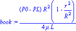
>	simplify( vz-book );

Solving for Concentration Gradient

Boundary Conditions:

 1) at z=0,  Ca = Cao

 2) at r=R, Ca = 0

 3) at r=0,  Ca = finite

Assumptions:

 5) Assume, for short distances z into the reactor, the concentration Ca differs from Cao only near the wall.

     In this region, the velocity profile is nearly linear.  See below for calculation of new linear velocity profile.

 Note: In example 12.2-2 they define vz(y) = vz_max*y/R for the linear profile with vz_max = (P0-PL)*R^2/(2*mu).  Since we have defined our vz_max as divided by 4*mu, we must define vz(y) = 2*vz_max*y/R to keep the constants straight.

 First we show that these two forms are identical.

>	vz_mine:=2*(P0-PL)*R^2/(4*mu)*y/R;

>	vz_book:=(P0-PL)*R^2/(2*mu)*y/R;

>	simplify( vz_mine - vz_book ); Therefore it is appropriate to use our definition of vz_max and vz.

The new motion equation therefore looks like this with the simplifications as given above.

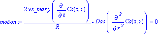
>	motion:=expand( (2*vz_max*y/R*diff(Ca(z, r), z)*r-Das*r*diff(Ca(z, r), `$`(r, 2)))/r = 0 );

Assumptions:

 6) In this region, we can neglect curvature terms

 7) Replace boundary condition (3) above with Ca=Cao at y=infinity

     => Introduce variable y=R-r

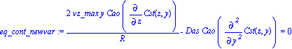
>	with(PDEtools): tr:={r=R-y,Ca(z,r)=Cao*Cst(z,y)}; eq_cont_newvar:=dchange(tr,motion,[y,Cst(z,y)]);

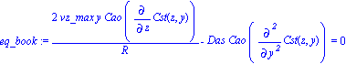
>	eq_book:=2*vz_max*y/R*diff(Cao*Cst(z,y),z)-Das*diff(diff(Cao*Cst(z,y),y),y)=0;

>	simplify( eq_book - eq_cont_newvar );

One thing to note, if you factor out Cao from both terms, you can divide both LHS and RHS through by Cao, and this eliminates this variable from the equation.  From this point on, Cst(z,y) will be replaced back to Ca(z,y).

Deriving a new differential equation

Boundary Conditions:

 1) at z = 0,         Ca = Cao

 2) at y = 0,         Ca = 0

 3) at y = infinity, Ca=Cao

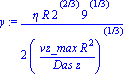
Because of the complexity of this ODE, we will seek a solution form of Ca/Cao = f(eta), where eta is given in the book as (y/r)*(2*vz_max*R^2/(9*Das*Z))^(1/3)

Here we will derive the dimensionless form of the ODE that is given in the book

>

restart;

Here is the ODE from before.

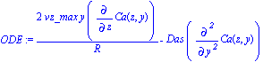
>	ODE:=2*vz_max*y/R*diff(Ca(z,y),z)-Das*diff(diff(Ca(z,y),y),y);

Here we define Ca as the books give it, moving Cao over to the other side.

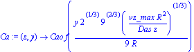
>	Ca:=(z,y)->Cao*f(y/R*(2*vz_max*R^2/(9*Das*z))^(1/3));

eq1 now is the original ODE with the new definition of Ca

>

eq1:=ODE;

By re-substituting back in for y we can eliminate it.

>	y:=eta*R/((2*vz_max*R^2/(9*Das*z))^(1/3));

Here I saw that the term vz_max *R^2/(Das*z)^(1/3) occurs a lot, so I divided through by this term.  eq2 has this simplification.  eq3 is just getting rid of all the constants.

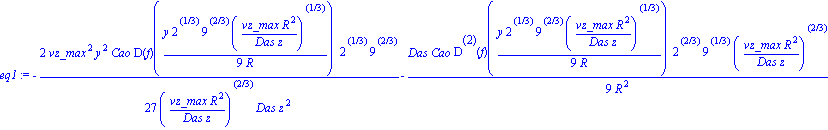
>	eq2:=simplify(-eq1*(vz_max*R^2/Das/z)^(1/3));

>	eq3:=simplify(-eq1*(vz_max*R^2/Das/z)^(1/3))*( 9*z/( Cao*vz_max*2^(2/3)*3^(2/3) ));

Solving the new ODE

The answer that Maple gives, although it may be correct, leaves a lot to be desired in terms of simplicity and understandablity (unfortunately).

>	s3:=dsolve( {eq3,f(0)=0,f(infinity)=1},f(eta) );

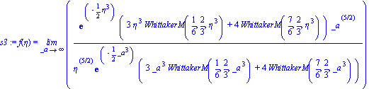
The book gives the following for the answer.  Plugging in shows that it does satisfy the ODE.

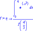
>	f:=eta->int( exp( -(x^3) ),x=0..eta )/Gamma(4/3);

Alas, the books solution is correct.  However, this still doesn't help anyone understand how they came up with the solution.  Since Maple seems to produce overly difficult answers, see the scanned in hand calculations.

>

eq3;

Plugging in some numbers

Here I'm going to make up some numbers just to see what the graph of Ca/Cao looks like.  Let's assume the diffusion coefficient for our system is something like 10^(-5).  Let's let the reactor be the same size of the oxidizers where I work, which must remain anonymous for proprietary reasons.  z=200ft*(12in/ft)*(2.54cm/1in)=6100 cm.  R=50ft=1524cm.  vz_max = 5*ft/s = 152cm/s

Given these conditions, calculate the distance away from the wall you must be to get Ca/Cao to be 0.5

Solution: Just plug in the numbers and do trial and error until Ca/Cao = 0.5

>	restart; Das:=10^(-5);z:=6100;R:=1524;vz_max:=152;

>

y:=.641;

>	eta_var:=evalf( y/R*(2*vz_max*R^2/(9*Das*z))^(1/3) );

>	Cao:=evalf( int( exp( -(x^3) ),x=0..infinity ) );

>	Ca:=evalf( int( exp( -(x^3) ),x=0..eta_var ) );

It is clear from this example that the distance away from the wall could have to be 0.641 for this model to apply.  Since we usually want to know something about the system farther than that off the wall, it is clear why more advanced methods are applicable.  See Matlab graph for various values of y and Ca/Cao.  Note that the region for y=0->1 is very linear.  Code for graph is attached at the end of the Maple session.

>

Ca/Cao;

Hand Calculations

Because the solution form involves the Whittaker functions, it is difficult to manipulate the functions in Maple.  Whittaker functions involve a sum of a bunch of terms and it is easier to see the development of the solution leaving the integrals in their unevaluated forms.

>

Code for Matlab Graph - Matlab Version

clear, clc

syms x

Das=10^(-5);
z=6100;
R=1524;
vz_max=152;

counter = 1

for y = 0.01:0.1:3
   eta_var=y/R*(2*vz_max*R^2/(9*Das*z))^(1/3);
   Cao=double( int( exp( -(x^3) ),x,0,inf ) );
   Ca=double( int( exp( -(x^3) ),x,0,eta_var ) );
   x_var(counter)=double(y);
   y_var(counter)=double(Ca/Cao);
   counter = counter + 1;
end

plot(x_var,y_var)