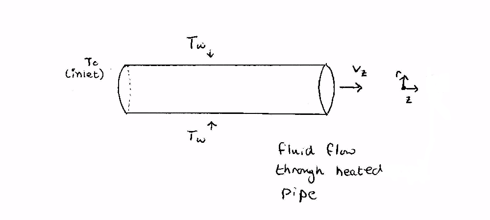
Illustrative Example 1: Temperature Distribution of Fluid Flowing Through a Pipe

One of the most common scenarios encountered in Transport involves some variation of fluid flowing through a pipe. In the common case that it is desired that the moving fluid be heated (or cooled), it is often of great practical importance to predict the temperature distribution of the moving fluid. This heating (or cooling) is often achieved by maintaining the pipe wall at a constant temperature.

There are serveral reasons that the temperature profile of the fluid may be of importance: If too high (or too low) a temperature is reached in the pipe, a phase change or other reaction may occur. A maximum (or minimum) temperature may need to be maintained to assure newtonian behavior, or many other reasons. Below the general approach to obtaining a temperature distribution for a moving fluid from the general energy equation is outlined:

Step 1: What is the geometry involved?

As most pipes are shaped as tubes (cylinders), it is obvious that cylindrical coordinates are the appropriate choice. Therefore, the equation of Energy in cylindrical coordinates should be used.

Step 2: What assumptions can be made?

The most common assumption in this type of problem is that the process is at steady state and that the pipe is long enough that edge effects can be ignored. We will also assume that the fluid is only moving in the z direction. Consequently, we will assume that the primary mode of energy transport in the z direction is by convection. As is usually the case, we will assume that we are concerned with a fluid such as water, and thus that viscous heating effects are negligible due to the fact the fluid is not extremely viscous. Finally, we assume that the wall is maintained at a constant temperatue and that the fluid enters the pipe with a uniform inlet temperature.

Step 3: What terms can be reasonably neglected?

This is perhaps the most important step in the initial analysis. Because of our assumption that there is only flow in the z direction, we see that all convection terms containing Vtheta and Vr equal zero. Additionally, since the process is at steady state, the time devivative drops out. If the fluid does not demonstrate large viscous heating, the viscous dissipation terms may also be ignored. Finally, since heat is being carried in (or out) of the fluid through the pipe walls, and we assume uniform pipe temperature, then the only conductive term that will remain in the equation is in the r direction. Begining with the general equation of energy in the appropriate coordinate system, the terms to be neglected are written with subscript [negligible] in the original equation:

> restart;

> >Generaleq:=rho*Cphat*(diff(T(r,theta,z,t),t)[negligible]+vr(r,theta,z,t)[negligible]*diff(T(r,theta,z,t),r)+(1/r)*vtheta(r,theta,z,t)[negligible]*diff(T(r,theta,z,t),theta)+vz(r,theta,z,t)*diff(T(r,theta,z,t),z))=k*((1/r)*diff((r*diff(T(r,theta,z,t),r)),r)+(1/r^2)*diff(T(r,theta,z,t),theta,theta)[negligible]+diff(T(r,theta,z,t),z,z)[negligible])+mu*phi[negligible];

At this point the remaining terms can be writen out. Examination of this equation may help determine what boundry conditions are appropriate and what further simplifications can be made. Starting with the equation of energy in cylindrical coordinates and neglecting the specified terms, the equation describing this process is:

> eq1:=rho*Cphat*vz(r,theta,z)*diff(T(r,theta,z),z)=k*((1/r)*diff((r*diff(T(r,theta,z),r)),r));

Going back to the considerations on geometery, in this process the Temperature and velocity in the pipe will have no dependence on theta (flow in the top half of the pipe assumed to be the same as in the bottom, etc.).

Then the final differential equation describing the process is:

> eq2:=rho*Cphat*vz(r,z)*diff(T(r,z),z)=k*((1/r)*diff((r*diff(T(r,z),r)),r));

The last consideration involves determining the boundry conditions in order to proceed to the solution.

Step 4: What are the boundry conditions?

At this point, it can be seen that the equation is second order in r and first order in z. Therefore, the solution requires two boundry conditions in r and one in z. Starting with the r direction, the most obvious condition is that since the temperature of the wall is constant, the heat flux in at the wall will likewise be constant.

at r=R

> BC1:=k*diff(T(r,z), r)=q[o] (constant);

Next, using some physical intuition, it can be seen that the temperature should not be infinite at r=0. This is of concern because teh equation contains a 1/r term.

> T(r=o):=finite;

Finally, going back to the assumptions, we assumed that whereever this fluid came from, it entered this pipe at a uniform temperature. therefore, the final boundry condition is:

> T(z=o):=To;

Now that a simplified form of the equation has been obtained and the appropriate number of boundry conditions have been specified, the system can be solved to obtain the desired temperature distribution! Such a solution can be obtained by combining variables into dimensionless form to reduce the number of variables and integrated over the appropriate range, as done in BS&L Chapter 11.