Section 18.6 ˆ Diffusion Into a Falling Liquid Film
CENG
402 Project By Jim Germanese, Spring 2002
Discussion of
situation:
<![if
!supportEmptyParas]> <![endif]>
 <![endif]>
<![if
!supportEmptyParas]> <![endif]>
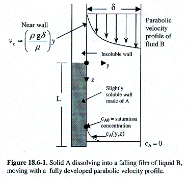
Liquid
B is flowing in laminar motion down a vertical wall as shown in
Figure 18.6-1 above. The
film begins far enough up the wall so that vz depends only
on y for z “ 0.
For 0 < z < L the wall is made of species A
that is slightly soluble in B.
<![if
!supportEmptyParas]> <![endif]>
For
short distances downstream, species A will not diffuse very far into
the falling film. That
is, A will be present only in a very thin boundary layer near the
solid surface. Therefore the diffusing A
molecules will experience a velocity distribution that is
characteristic of the falling film right next to the wall, y = 0.
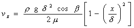
The general velocity distribution for the case of a fluid
moving down a wall is given by
<![if
!supportEmptyParas]> <![endif]>
 <![endif]>
<![if
!supportEmptyParas]> <![endif]>
where
x is measured from the outer edge of the film and b is the angle the wall makes with
the direction of gravity. Applied
to our case, cos b = 1 and x = d - y.
Thus, for our case, the velocity profile is as follows,
<![if !vml]>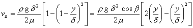 <![endif]>
<![if
!supportEmptyParas]> <![endif]>
At
and adjacent to the wall, (y/d)2 << (y/d), so the velocity
is, to a very good approximation,
vz
= (rgd/m)y º ay. The general differential
equation that governs this situation for short distances downstream,
given by Eq. 18.5-6, is
<![if
!supportEmptyParas]> <![endif]>
<![if
!supportEmptyParas]> <![endif]>
again,
with x measured from the edge of the film inward. This simplifies, in our case, to
<![if
!supportEmptyParas]> <![endif]>
<![if !vml]>
<![endif]>
![]()
<![if
!supportEmptyParas]> <![endif]>
The
applicable boundary conditions are as follows,
<![if
!supportEmptyParas]> <![endif]>
B.C.
1:
at z = 0,
cA = 0
B.C.
2:
at y = 0,
cA = cA0
B.C.
3:
at y = ¥,
cA = 0
<![if
!supportEmptyParas]> <![endif]>
cA0
represents the
solubility of A in B. The
third boundary condition comes from the assumption that molecules of
A penetrate only slightly into the film, which means that they cannot
distinguish between the boundary condition given here and the
expected boundary condition (at y = d, ¶cA / ¶y = 0).
<![if
!supportEmptyParas]> <![endif]>
Due to the form of the boundary conditions, a change in variables is used to simplify the problem.
<![if
!supportEmptyParas]> <![endif]>
> restart;
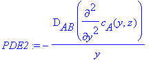
Splitting up the partial differential equation into two
parts,
> PDE1:=a*diff(c[A](y,z),z);
> PDE2:=(-D[AB]/y)*diff(c[A](y,z),y,y);
Changing variables or both pieces of the partial
differential equation,
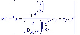
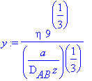
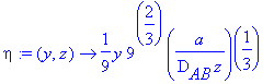
> tr1:={c[A]=c[A0]*f,z=((y/eta)^3)*(a/(9*D[AB]))};
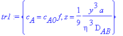
> tr2:={c[A]=c[A0]*f,y=eta/((a/(9*D[AB]*z))^(1/3))};
> with(PDEtools):
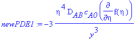
> newPDE1:=dchange(tr1,PDE1,[eta,f(eta)]);
> newPDE2:=dchange(tr2,PDE2,[eta,f(eta)]);
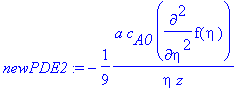
The sum of newPDE1 and newPDE2 is the left-hand-siide of
the original equation. So, newPDE
represents an unsimplified dimensionless form of the original partial differential equation.
> newPDE:=newPDE1+newPDE2=0;
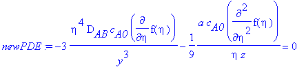
Simplifying newPDE,
> y:=eta/((a/(9*D[AB]*z))^(1/3));
> newPDE;
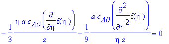
> ODE:=simplify(((-9*eta*z)/(a*c[A0]))*newPDE);
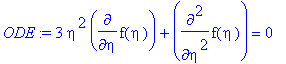
Thus, ODE, by inspection, matches Equation 18.6-6.
Attempting to solve the
ordinary differential equation,
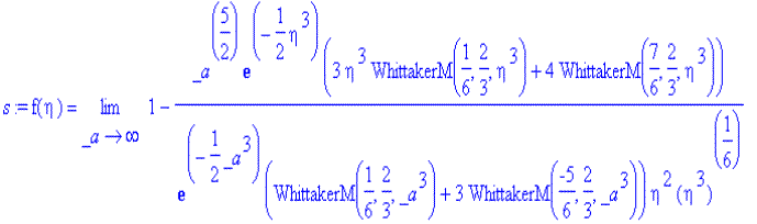
> s:=dsolve({ODE,f(0)=1,f(infinity)=0},f(eta));
 <![endif]>
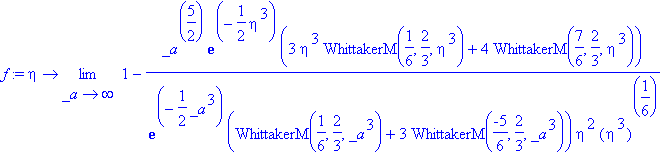
> assign(s);f:=unapply(f(eta),eta);
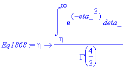
Checking this result with Equation 18.6-8,
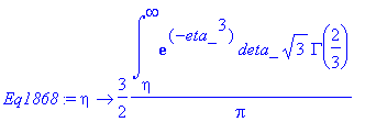
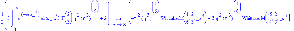
> Eq1868:=eta->int(exp(-eta_^3),eta_ = eta .. infinity)/GAMMA(4/3);

> simplify(Eq1868(eta));
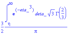
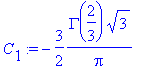
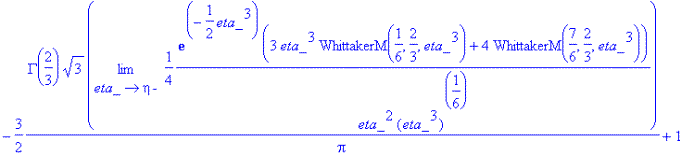
> Eq1868:=eta->3/2*int(exp(-eta_^3),eta_ = eta .. infinity)*sqrt(3)*GAMMA(2/3)/Pi;
> simplify(expand(Eq1868(eta)-f(eta)));

As this will not simplify, we must check our solution by
another method. To check our solution, we can plug the above relation
for f(eta) into the governing differential equation to see if it
satisfies it. We can then check the boundary conditions to ensure
that those hold as well. So, plugging back into the governing
differential equation,
> simplify(expand(simplify(diff(f(eta),eta,eta)+3*eta^2*diff(f(eta),eta))));
Therefore, the above relation for f(eta) satisfies the
ordinary differential equation. Unfortunately, the above function
cannot be evaluated using the evalf Maple function. Thus, the
boundary conditions cannot be checked. Yet, a different approach can
be used and verified
in Maple.
Using Equation C.1-9,
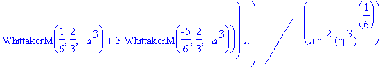
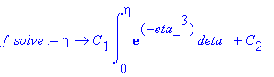
> f_solve:=eta->C[1]*int(exp(-eta_^3),eta_=0...eta)+C[2];
Applying the boundary conditions,
> BC1:=f_solve(0)=1;
Thus, C2 = 1. Further,
> eq2:=f_solve(infinity)=0;
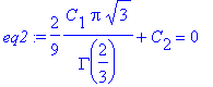
> C[2]:=1;
> C[1]:=solve(eq2,C[1]);
So, plugging in the above integration constants,
> f_solve(eta);
 <![endif]>
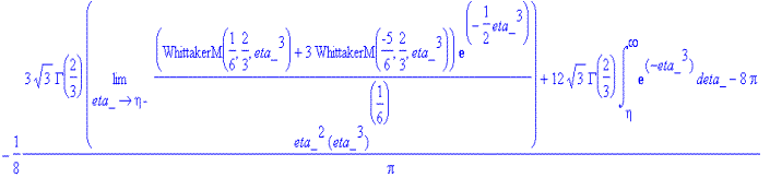
Checking to see if f_solve(eta)=Eq1868(eta),
> simplify(f_solve(eta)-Eq1868(eta));
 <![endif]>
As this won't simplify, a different method must be used
to verify that f_solve(eta) gives the correct relation.
Checking that f_solve(eta) matches the governing ordinary differential equation and the boundary conditions,
> diff(f_solve(eta),eta,eta)+3*eta^2*diff(f_solve(eta),eta);
Thus, f_solve(eta) fits the governing differential
equation. Checking the first boundary condition (i.e. that f(0)=1),
> f_solve(0);
Checking the second boundary condition (i.e. that
f(infinity)=0),
> f_solve(infinity);
Thus, both boundary conditions check. Therefore,
f_solve(eta) solves the differential equation. Now checking that
Equation 18.6-8 is a valid solution by a similar method,
> diff(Eq1868(eta),eta,eta)+3*eta^2*diff(Eq1868(eta),eta);
> Eq1868(0);
> Eq1868(infinity);
Thus, Equation 18.6-8 is a valid solution and is
equivalent to f_solve(eta).
Determining the local mass flux at the wall, starting with Equation 18.6-8,
> restart;
> eta:=(y,z)->(y*(a/(9*D[AB]*z))^(1/3));
> Eq1868:=eta->int(exp(-eta_^3),eta_ = eta .. infinity)/GAMMA(4/3);

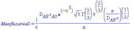
> Massfluxatwall:=-D[AB]*c[A0]*diff(Eq1868(eta),eta)*diff(eta(y,z),y);
To calculate the mass flux at the wall, this quantity
must be evaluated at y = 0 and, thus, eta = 0. So,
> eta:=0;Massfluxatwall;
Checking with Equation 18.6-9,
> Eq1869:=((D[AB]*c[A0])/(GAMMA(4/3))*((a/(9*D[AB]*z)))^(1/3));
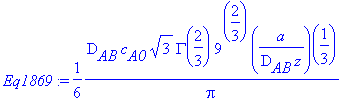
> simplify(Massfluxatwall-Eq1869);
Thus, Massfluxatwall matches Equation 18.6-9.
Now, determining the molar flow of A across the entire mass transfer surface at y = 0,
> restart;
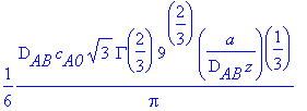
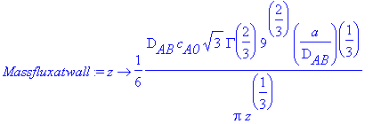
> Massfluxatwall:=z->(1/6*D[AB]*c[A0]*sqrt(3)*GAMMA(2/3)*9^(2/3)*(a/(D[AB]))^(1/3)/Pi)/(z^(1/3));
> Totalmolarflow:=int(int(Massfluxatwall(z),z=0...L),x=0...W);

Comparing this result with Equation 18.6-10,
> Eq18610:=((2*D[AB]*c[A0]*W*L)/(GAMMA(7/3)))*(a/(9*D[AB]*L))^(1/3);
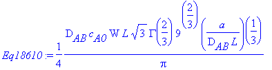
> simplify(Totalmolarflow-Eq18610,assume=positive);
Thus, the above relation matches Equation 18.6-10 and
represents the molar flow of A across the entire mass
transfer surface at y = 0.
<![if
!supportEmptyParas]> <![endif]>
An
Example:
Consider a slab 1 meter tall and 1 meter wide of
trinitrotoluene, or TNT, which is used in explosives. A film of water
.5 cm wide is falling down the slab. TNT is slightly soluble in water, with a solubility of 0.035g / 100g of water. Assume that the temperature is 20 degrees C and that the solubility of the TNT-water solution can be approximated as the viscosity of water at 20 degrees C. Plot the normalized (cTNT/cTNT0) concentration gradient half way down the slab. Also, calculate the local mass flux of TNT at the wall halfway down the slab and the total molar flow of TNT across the entire slab.
> restart;
Calculating the concentration gradient when z = .5
meters, using Equation 18.6-8,
> Eq1868:=eta->int(exp(-eta_^3),eta_ = eta .. infinity)/GAMMA(4/3);
Calculating a,
> a:=(rho[water]*g*delta)/(mu[water]);
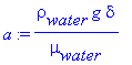
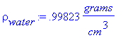
> rho[water]:=.99823*(grams/cm^3);g:=981*(cm/sec^2);delta:=.5*cm;mu[water]:=.01*(grams/(cm*sec));
![]()
![]()
> simplify(a);
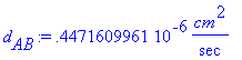
Calculating diffusivity, denoted d[AB] using
Equation 17.4-8, omitting units for the intermediate values (all in
cgs, temp. in K),
> d[AB]:=(7.4/10^8)*((phi[water]*M[water]*T)^(.5)/(mu*V[TNT]^(.6)));
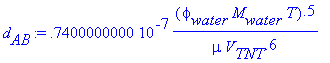
> phi[water]:=2.6;M[water]:=18.02;T:=293.15;mu:=1;V[TNT]:=140;
![]()
![]()
![]()
![]()
> d[AB]:=d[AB]*(cm^2/sec);
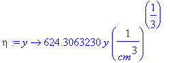
Defining function for eta,
> eta:=y->y*(((48963.18150*1/sec)/(9*(.4471609961e-6*cm^2/sec)*50*cm))^(1/3));
Calculating eta when y=delta=.5 cm,
> eta(.5*cm);
Plotting normalized concentration profile at z = .5
meters,
> with(plots):
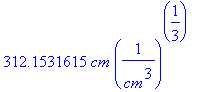
> plot(Eq1868(eta),eta=0...312.1531615);
Plotting error, exponent too large
As Maple cannot plot when y=delta=.5 cm, attempting a
smaller range, from eta = 0 to eta = 6.24306232
(.01 cm from the wall),
> plot(Eq1868(eta),eta=0...6.24306232);
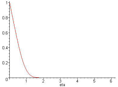
This plot is what we expect. The concentration of TNT at
the wall, when eta = 0, equals the solubility of TNT in water.
As one moves further from the wall, the concentration of
TNT falls off rapidly.
Calculating the local mass flux at the slab halfway down the slab (at z = .5 meters), using Equation 18.6-9,
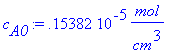
>mu:='mu':mu[water]:=.01*(grams/(cm*sec)):c[A0]:=(3.4938/10^4)*(grams/cm^3):a:=(rho[water]*g*delta)/(mu[water]):z:=50*cm:Localwallflux:=((d[AB]*c[A0])/(GAMMA(4/3))*(a/(9*d[AB]*z))^(1/3));
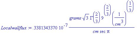
> Localwallflux:=evalf(simplify(Localwallflux*(cm)/(1/cm^3)^(1/3)));
Thus, this gives the mass flux of TNT at the wall
halfway down the wall.
Calculating the total molar flow of TNT across the entire slab, using Equation 18.6-10,
> W:=100*cm;L:=100*cm;c[A0]:=1.5382e-6*(mol/cm^3);Molarflow:=((2*d[AB]*c[A0]*W*L)/(GAMMA(7/3)))*(a/(9*d[AB]*z))^(1/3);
![]()
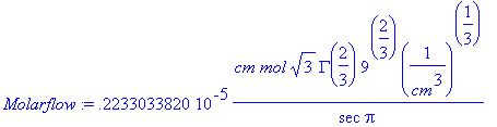
> Molarflow:=evalf(Molarflow/(cm*(1/cm^3)^(1/3)));
This is the total molar flow rate of TNT into water for
the entire slab.