CENG 402 Final Project
George Wells and Burt Kobylivker
April 25, 2002

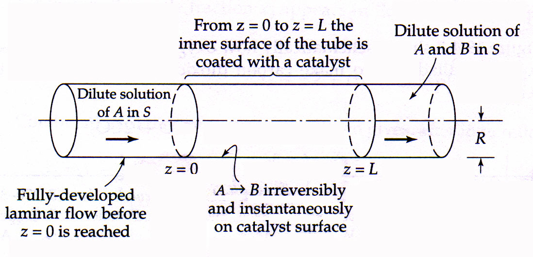
EXAMPLE 19.4-2 Concentration Profile in a Tubular Reactor

In the catalytic tubular reactor shown above, a dilute solution of solute A in a solvent S is in fully developed, laminar flow in the region z<0. When it encounters the catalytic wall in the region 0<=z<=L, solute A is instantaneously and irreversibly rearranged to an isomer B. We will write the diffusion equation appropriate for this problem, and find the solution for short distances into the reactor. Also, we will assume that the flow is isothermal and neglect the presence of B.

> restart;

The flowing liquid will always be very nearly pure solvent S. The product rho*Das can be considered constant, and the diffusion of A in S can be considered by a steady state version of the the continuity equation in terms of molar concentration (equation B.11.2). Note that the presence of a small amount of the reaction product B is ignored.

> equcont:=vz(r)*diff(c[A](r,z),z)=Das*(1/r*diff(r*diff(c[A](r,z),r),r)); Equation 19.4-18: steady state equation of continuity ignoring small amount of reaction and axial diffusion, which can be neglected with respect to axial convection.

Determination of Velocity Distribution in a Horizontal Cylinder of radius R with laminar, fully developed flow

> Pin:=2*pi*r*dr*P0; Pressure in

> Pout:=2*pi*r*dr*PL; Pressure out

> Tauforce:=r->taurz(r)*2*pi*r*L; Viscous force in z direction at constant r

> Tauforce(r); Viscous force at r

> Tauforce(r+dr); Viscous force at r+dr

This a momentum balance with the pressure and shear stress forces. Velocity is only in the axial or Z-Direction so Vr=Vtheta=0. Vz is only a function of the distance "r."

> Momeq:=limit((Pin-Pout+Tauforce(r)-Tauforce(r+dr))/(2*pi*L*dr),dr=0); Momentum balance over cylinder of length r, assuming P is independent of r and theta and linearly dependent on z

> sol:=dsolve({Momeq,taurz(0)=finite},taurz(r)); Momentum flux cannot be infinite at the axis of the tube.

> taurz:=(r)-> -mu*D(Vz)(r); Substitution of Newton's Law of Viscosity

> sol;

> sol1:=dsolve({sol,Vz(R)=0},Vz(r)); B.C. Vz=0 at the radius of the cylinder (This is the no slip condition)

> finaleq:=simplify(sol1); The velocity equation from maple.

> finaleq:=-1/4*(r^2*P0-r^2*PL-R^2*P0+R^2*PL)/(L*mu);

> book:=(P0-PL)*R^2/(4*mu*L)*(1-(r/R)^2); Book velocity equation.

> simplify(book-finaleq);

Thus, the book equation for the velocity distribution in a horizontal cylinder is the same as that from Maple.

The maximum velocity occurs when r=0 providing vzmax=(P0-PL)*R^2/(4*mu*L)

> vz:=r->vzmax*(1-(r/R)^2); Velocity equation incorporating Vzmax.

> equcont; equation 19.4-20

The equation above is to be solved with the boundary conditions

B.C. 1: at z=0, cA=cA0

B.C. 2: at r=R, cA=0

B.C. 3: at r=0, cA=finite

For short distances z into the reactor, the concentration cA differs from cA0 only near the wall. The following three assumptions are accurate in the limit as z->0:
1. Curvature effects may be neglected and the problem treated as though the wall were flat; we will introduce the variable y=R-r, where y is the distance from the wall
2. The fluid may be regarded as extending from the (flat) catalyst surface (y=0) to y=infinity

3. The velocity profile may be regarded as linear, with a slope given by the slope of the parabolic velocity profile at the wall: vz(y)=2*vzmax*y/R
This is the way the system would appear to a tiny "observer" who is located within the very thin shell of fluid near the wall. To this observer, the wall would seem flat, the fluid would appear to be of infinite extent, and the velocity profile would seem to be linear. (See example 12.2-2 for a detailed discussion of this method for treating the entrance region of the tube.)

> with(PDEtools,dchange);

> transf:={r=R-y};

> Newde:=expand(dchange(transf,equcont,[y])); Changing variable from r to y.

Assuming a linear velocity profile, the term on the left which involves y^2/R^2 can be neglected. The first term on the right is neglected because curvature affects are ignored here. Rearranging and noting that R is a constant, we obtain:

> equ:=y*diff(c[A](y,z),z)-R/2/vzmax*Das*diff(diff(c[A](y,z),y),y); Rearranged Equation 19.4-24

With the boundary conditions
B.C. 1: at z=0, cA=cA0
B.C. 2: at y=0, cA=0
B.C. 3: at y=infinity, cA=cA0
This problem can be solved by the method of combination of independent variables by seeking a solution of the form cA/cA0=f(eta), where eta=(y/R)(2*vxmax*R^2/9*Das*z)^1/3.

> c[A]:=(y,z)->c[A0]*f(y/R*(2*vzmax*R^2/(9*Das*z))^(1/3)); Nondimensionalizing, assuming solution of the form cA/cA0=f(eta)

> equ1:=equ;

> y:=eta*R/((2*vzmax*R^2/(9*Das*z))^(1/3)); Substituting for y;

> equ2:=simplify(equ1*(-18)/6^(2/3)/c[A0]/R*z*(vzmax*R^2/Das/z)^(1/3)); This is easily integrable by equation C.1-9

> equ3:=dsolve({equ2,f(0)=0},f(eta)); Maple has trouble with it, though

> equ3:=dsolve({equ2,f(0)=0, f(infinity)=1},f(eta)); Especially if we try to solve with both boundary conditions

> f:=eta->int(exp(-eta1^3),eta1=0...eta)/Gamma(4/3); Here is the book's answer. The Gamma function, which is a constant when evaluated at any number, is described in section C.4.

> equ2; It satisfies the DE and hence is a solution to the problem.

NUMERICAL EXAMPLE
According to Bird, Stewart, and Lightfoot, a particularly attractive reaction is the reduction of ferricyanide ions on metallic surfaces in which ferricyanide and ferrocyanide take the place of A and B in the above development. This electrochemical reaction is quite rapid under properly chosen conditions. Since the reaction only involves electron transfer, the physical properties of the solution are almost entirely unaffected.

> Das:=7.6*10^(-6)*cm^2/s; The diffusion coefficient of ferricyanide in a 0.1M aqueous solution of KCl. This value was obtained from this website.
z:=100*cm; y:=.01*cm; R:=3*cm; vzmax:=1000*cm/s; These are arbitrary pipe parameters. The point we are analyzing corresponds to 100cm into 6 cm diameter catalysis pipe, 0.01cm from the wall, where the maximum flow velocity is 1000cm/s.

> eta:=evalf(y/R*((2*vzmax*R^2/(9*Das*z))^(1/3)));

> Gamma(4/3):=evalf(int(exp(-eta1^3),eta1=0...infinity)); Evaluating the gamma function.

> equ:=evalf(f(eta))=ca/ca0; The ratio between the concentration at the given reactor parameters and the initial concentration is given below.

Concentration Profile ca/ca0 as a Function of the Distance from the Reactor Wall at 100 cm into Reactor Tube

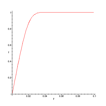
Maple code for generation of this plot is given here.