![[Maple Math]](images/maplesheet5.gif)
Table of Contents:
1. Introduction
2. Theoretical Basis
3. Empirical Calculations
4. Summary of Results
5. Conclusion
6. References
Due to the lack of a completely accurate model of liquids, the calculation of liquid viscosity is difficult. Although some models can accurately represent certain types of liquids (e.g. liquid metals, polar compounds), there is no model that encompasses all types of liquids. This project will examine one commonly used model, developed by Eyring, as well as develop a program that uses empirical data to predict liquid viscosities over a wide range of temperatures. Eyring's model is one of the earliest attempts at predicting liquid viscosities and has the least sound theoretical basis. However, later theories based on the principals of statistical mechanics have done little to improve on the accuracy of Eyring's liquid viscosity predictions. Since all of the current models are in error by as much as thirty to fifty percent, the viscosities predicted can only be used in very rough back of the envelope calculations. These calculations, however, are still useful because they require no experimentation beyond the determination of the boiling point and the liquid molar volume (both of which are very easy to measure). In industrial applications, empirical formulas are generally used for more accurate predictive results. Hence, we have developed a matlab program that uses a four parameter empirical model to predict liquid viscosity for several common liquids included in the start301 database.


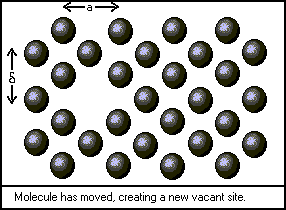
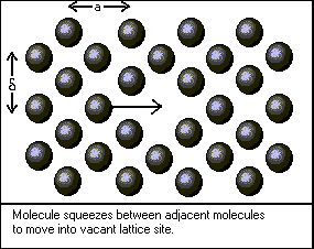
The first step in developing a theoretical model of viscosity is to define the behavior of a single molecule in a stationary fluid. The figures above depict the restricted fashion in which a molecule of liquid can move. Although each molecule vibrates within the space available to it, translational motion occurs less often. To squeeze past its neighbors, the molecule must obtain a certain activation energy, denoted by deltaGo/N. Bird, Stuart, and Lightfoot give the frequency of this event as
![[Maple Math]](images/maplesheet5.gif)
![[Maple Math]](images/maplesheet7.gif)
It is evident that the magnitude of the effect of sheer stress on jump frequency is inversely proportional to the distance between the molecules and the temperature. Once the motion of a single molecule has been modeled, it is possible to describe that of the whole fluid. The velocity of a given cross section of liquid is equivalent to the net frequency of forward and reverse jumps multiplied by the distance traveled per jump. If the velocity gradient over delta is taken to be linear, we find that
![[Maple Math]](images/net1.gif)
When substituting the expressions for nu(+) and nu(-) into the above expression, after expanding using a Taylor series expansion is
![]()
To see further details, follow the link to the Maple worksheet or refer to Section 1.5 in BSL(2001).
Sample Calculation from Theory
Since the simpler theoretical models for liquid viscosity do not
generate reasonably accurate results, empirical formulas are often
used in their place. The matlab code below calculates viscosities
using four parameter model of the form:
ln(viscosity)=A+B/T+C*T+D*T^2.
Data for eighteen liquids have been entered into the start301 database,
and the Matlab
Program can be used to predict liquid viscosities. Refer to the sample
calculation below.
Sample Calculation
Here are your compounds' formulae and names:
No. Formula  Name
----------------------------------------
  1 C6H6     benzene

Here are your reactions:
----------------------------------------
No reactions given

Enter the number of streams: 1

The variables for your compounds have now been created,
>> liqmucalc(20)

mu =

    0.6516
|
Substance |
Temperature (degC) |
Experimental Viscosity (cp) |
Emperical Viscosity (cp) |
Eyring Viscosity |
Emperical % Error |
Eyring % Error |
|---|---|---|---|---|---|---|
|
Water |
0 |
1.787 |
1.726 |
3.978 |
3.4 |
122.6 |
|
|
20 |
1.002 |
1.018 |
2.792 |
1.6 |
178.6 |
|
Diethyl Ether |
0 |
0.283 |
0.275 |
0.276 |
2.8 |
2.5 |
|
25 |
0.224 |
0.214 |
0.193 |
4.5 |
14.0 |
|
|
Bromine |
25 |
0.744 |
0.934 |
0.535 |
25.5 |
28.0 |
|
Benzene |
20 |
0.649 |
0.652 |
0.436 |
0.5 |
32.8 |
|
Ethanol |
0 |
1.786 |
1.720 |
0.908 |
3.7 |
49.2 |
|
25 |
1.074 |
1.041 |
0.603 |
3.1 |
43.9 |
|
|
50 |
0.694 |
0.670 |
0.426 |
3.5 |
38.6 |
|
|
Sulfuric Acid |
25 |
25.5 |
20.1 |
18.5 |
21.2 |
27.4 |
As can be seen in the above table, the theoretical predictions differ from the actual viscosities by 20-50% in most cases, with the predictions for water off by over 100%. The empirical predictions are much better, with deviations from the actual values usually less than 10%. Thus, although the theory does provide a general understanding of the phenomena that are occurring in a liquid system, the inaccuracy of the predictions show that much work is still necessary to create a comprehensive theory of liquid behavior.