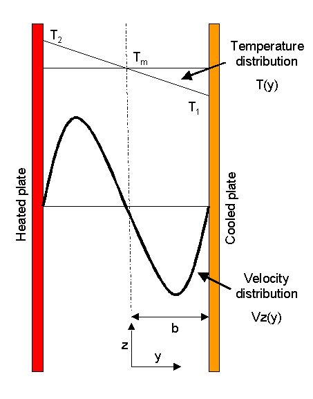
Section 9.9 --> Free Convection
In this section the problem of free convection of a fluid between 2 paralell walls of infinite lengths and different temperatures was studied. The fluid had a density of rho, a viscosity of mu, and was between walls a distance of 2b apart. The temperature of the cool wall, at b, is T1 and the temperature of the hot wall, at -b, is T2. It is assumed the the flow of fluid up is equal to the flow of fluid down.
> restart;
An energy balance over a shell paralell to the plates with a thickness of Delta y can be made resulting in equation 9.9-1. The temperature is a function of the horizontal component y.
> eqn1:=k*diff(diff(T(y),y),y)=0;
![[Maple Math]](images/mondro1.gif)
To obtain the temperature profile the above equation is solved for the boundary conditions at the surfaces of the plates. The temperatures at y = b is T1 and at y = -b is T2.
> dsolve({eqn1,T(b)=T1,T(-b)=T2},T(y)):
> assign(%): T:=unapply(T(y),y);
![]()
This is equal to the the solution equation 9.9-4.
Defining Delta T, the differences between wall temperatures, and Tm the arithmetic mean of the temperatures as:
> Delta[temp] := T2-T1; Tm := (T1+T2)/2;
![]()
![]()
By taking a momentum balance over the the same control volume with a thickness of Delta y, the velocity distribution in the z direction [equation 9.9-5] is obtained.
> eqn2:=mu*diff(diff(vz(y),y),y) = diff(p(z),z)+rho[T]*g;
![[Maple Math]](images/mondro5.gif)
rhoT can be expressed as a Taylor series expansion in temperature (t) with respect to a reference temperature Tref. Only the first two terms are considerd [equation 9.9-6].
> rho[T]:= rho[ref]-rho[ref]*beta[ref]*(t-T[ref]);
![]()
Substitution of the density results in equation 9.9-7;
> eqn2;
![[Maple Math]](images/mondro7.gif)
It is also assumed the pressure variance is only from the weight of the fluid. The pressure can be solved for by:
> eqn3:= diff(p(z),z)= -rho[ref]*g;
> dsolve({eqn3,p(0)=0},p(z)):
> assign(%); p:=unapply(p(z),z);
![]()
![]()
Substitution of pressure back into equation 9.9-7 results in equation 9.9-8.
> eqn2:=collect(simplify(eqn2),{g,rho[ref],beta[ref]});
![[Maple Math]](images/mondro10.gif)
This equation implies that the viscous forces are balances by the boyant forces. Inserting the temperature distribution derived earier results in equation 9.9-9
> t:=T(y): eqn2;
![[Maple Math]](images/mondro11.gif)
This equation is solved with the boundary condition that the velocity of the gas is 0 at the surface of the wall. Solving this equation using newer Maple features such as PDEtools was attempted, but the correct solutions were not obtained by these methods.
> simplify(dsolve({eqn2,vz(b)=0,vz(-b)=0},vz(y))):
> assign(%); vz:=unapply(vz(y),y);
![]()
![]()
Dimentionless parameters were introduced to the equation.
> y:=eta*b; T[ref]:= Tm-A*Delta[temp]/6;
![]()
![]()
The results were simplifified to an equation eqivalent to equation 9.9-12.
> vz(eta) := simplify(collect(vz(y),{eta,beta[ref],rho[ref],g,b,mu}));
![[Maple Math]](images/mondro16.gif)
The volume flow in the z direction must be 0. Equation 9.9-12 is integrated with repect to dimentionless position from one wall to the other, set equal to 0 and solved for A.
> eqn4:= int(vz(eta),eta=-1...1)=0;
> A:= solve(evalf(eqn4),A);
![[Maple Math]](images/mondro17.gif)
![]()
Since A is equal to zero, the mean temperature is equal to the reference temperature. This changes equation 9.9-12 to an equation equivalent to 9.9-15.
> Vz(eta):= simplify(collect(vz(y),{beta[ref],rho[ref],g,b,mu,eta}));
![[Maple Math]](images/mondro19.gif)
This velocity distrubution is the result of buoyancy forces resulting in temperature differences in the system.
Equation 9.9-15 can be rewritten interms of dimentionless velocity (phi), dimentionless legnth (eta) and the Grashoff number (Gr). When this is simplified, it results in equation 9.9-16 as listed in B.S.L.
> phi:=b*Vz*rho[ref]/mu;
> Gr:=rho[ref]^(2)*beta[ref]*g*b^3*Delta[temp]/mu^2; Vz:=Vz(eta):
> eqn6:= simplify(phi/Gr): phi:='phi': Gr:='Gr': phi:=Gr*eqn6;
![[Maple Math]](images/mondro20.gif)
![[Maple Math]](images/mondro21.gif)
![]()
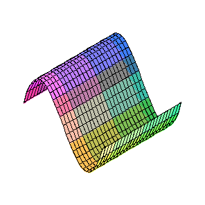
Arbritarily selecting a value for Gr, the plot of the dimentionless equation looks similar to the velocity distribution in the illustration.
> Gr:=12:plot(phi,eta=-1...1);plot3d(phi,m=0..1,eta=1...-1);
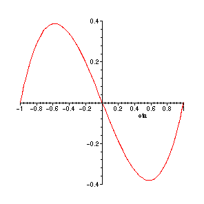
The points where the velocity is the greatest in each direction can be calculated.
> solve(diff(phi,eta)=0);
![]()
The points where the velocity is 0 can also be solved for. These points agree with the bounday conditions given in the problem.
> solve(phi=0,eta);
![]()