> restart;

> Sc:=T->Sc1*(T-T0)/(T1-T0); The volume rate of thermal energy produced by reactions is Sc. This is a simplification assuming a linear temperature independence.

> Qcond:=z->pi*R^2*qz(z); Thermal energy by conduction through the reactor at a point z.

> Qconv:=z->pi*R^2*rho1*v1*Cp*(T(z)-T0); Thermal energy by convection through the reactor at a point z.

> LHS:=limit((Qcond(z+dz)-Qcond(z)+Qconv(z+dz)-Qconv(z))/pi/R^2/dz,dz=0); Energy balance across a segment of length delta z. Taking the limit as delta z goes to 0 gives a differential equation.This equation does not include the energy production term.

> qz:=z->-keff*D(T)(z); Subsitutes Fourier's Law into differential equation.

> eq1:=simplify(LHS=0); Equation for Zone 1.

> eq2:=simplify(LHS=Sc(T(z))); Adds the term for heat generated by chemical reaction within the reactor.

> eq3:=simplify(LHS=0); Equation for Zone 3.

> with(PDEtools,dchange); Loads the dchange command.

> transf1:={z=Z*L,T(z)=Theta1*(T1-T0)+T0}; Sets up the dimensionless variable transfer vectors for the three sections of the reactor. These are used with dchange.

> transf2:={z=Z*L,T(z)=Theta2*(T1-T0)+T0};

> transf3:={z=Z*L,T(z)=Theta3*(T1-T0)+T0};

> eq1b:=dchange(transf1,eq1,[Theta1(Z),Z]):

> eq2b:=dchange(transf2,eq2,[Theta2(Z),Z]):

> eq3b:=dchange(transf3,eq3,[Theta3(Z),Z]):

Substitute for the other two dimensionless quantities, which are parameters for the system.

> v1:=B*keff/rho1/Cp/L:

> Sc1:=rho1*v1*Cp*(T1-T0)*N/L:

The dimensionless differential equations for each of the three zones simplified so that they are similar to BSL equations 9.5-23-25

> eq1c:=simplify(eq1b*L^2/B/keff/(-T1+T0));

> eq2c:=simplify(eq2b*L^2/B/keff/(-T1+T0));

> eq3c:=simplify(eq3b*L^2/B/keff/(-T1+T0));

Using dsolve to solve the differential equations.

> s1:=dsolve(eq1c,Theta1(Z));

>

> assign(s1); Theta1:=unapply(Theta1(Z),Z):

> _C1:=1; _C2:=c2; We know that c1=1 because at Z=-infinity, T is equal to T1 meaning that Theta equals 1.

> s2:=dsolve(eq2c,Theta2(Z));

> _C3:=c3; _C4:=c4;

> assign(s2); Theta2:=unapply(Theta2(Z),Z);

> s3:=dsolve(eq3c,Theta3(Z));

> assign(s3); Theta3:=unapply(Theta3(Z),Z);

> _C6:=0; _C5:=c5; We know that c6=0 because at z=infinity, T is finite.

> con:=solve({Theta1(0)=Theta2(0),D(Theta1)(0)=D(Theta2)(0),Theta2(1)=Theta3(1),D(Theta2)(1)=D(Theta3)(1)},{c2,c3,c4,c5}); Solving for the remaining constants using the given boundary conditions.

> assign(con);

The three final solutions are very complicated in Maple.

> simplify(Theta1(Z));

> simplify(Theta2(Z));

> simplify(Theta3(Z));

>

Some example cases using different values for the parameters B and N.

> B:=8;N:=1;

>

> PlotN11:=simplify(evalf(expand(Theta1(Z))));

>

> PlotN12:=simplify(evalf(expand(Theta2(Z))));

> PlotN13:=simplify(evalf(expand(Theta3(Z))));

> pN11:=plot(PlotN11,Z=-.6...0):

> pN12:=plot(PlotN12,Z=0...1):

> pN13:=plot(PlotN13,Z=1...1.3):

> with('plots'):

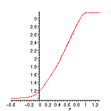
> display([pN11,pN12,pN13]); This generates a plot very similar to the one in BSL.

> N:=2;

> PlotN01:=simplify(evalf(expand(Theta1(Z))));

Error, (in Theta1) division by zero

> PlotN02:=simplify(evalf(expand(Theta2(Z))));

Error, (in Theta2) division by zero

> PlotN03:=simplify(evalf(expand(Theta3(Z))));

Error, (in Theta3) division by zero

> N:='N'; For N=2, we get a divide by 0 error. This can be solved by taking the limit as N goes to 2.

> PlotN21:=limit(simplify(evalf(expand(Theta1(Z)))),N=2);

> PlotN22:=limit(simplify(evalf(expand(Theta2(Z)))),N=2);

> PlotN23:=limit(simplify(evalf(expand(Theta3(Z)))),N=2);

> pN21:=plot(PlotN21(Z),Z=-.6...0):

> pN22:=plot(PlotN22(Z),Z=0...1):

> pN23:=plot(PlotN23(Z),Z=1...1.5):

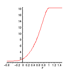
> display([pN21,pN22,pN23]); This plot is also identical to that shown in BSL.

> N:=4;

> PlotN41:=simplify(evalf(expand(Theta1(Z))));

> PlotN42:=simplify(evalf(expand(Theta2(Z))));

> PlotN43:=simplify(evalf(expand(Theta3(Z))));

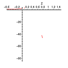
We find that with a value of B=8, that for values of N greater than 2 Maple gives an imaginary solution. This is because of the sqrt(-B(-B+4N)) term in our solutions. However these should cancel out to give a real answer.

> pN41:=plot(PlotN41(Z),Z=-.6...0):

> pN42:=plot(PlotN42(Z),Z=0...1):

> pN43:=plot(PlotN43(Z),Z=1...1.5):

> display([pN41,pN42,pN43]);

In the region in the reactor, the imaginary terms do not go away so we cannot generate a good plot. If we try the book's solutions a much better answer is obtained.

> m3:=1/2*B*(1-sqrt(1-4*N/B));

> m4:=1/2*B*(1+sqrt(1-4*N/B));

> T1book:=1+(m3*m4*(exp(m4)-exp(m3)))/(m4^2*exp(m4)-m3^2*exp(m3))*exp((m3+m4)*Z);

> Theta1bk:=simplify(expand(evalf(T1book)));

> T2book:=(m4*exp(m4)*exp(m3*Z)-m3*exp(m3)*exp(m4*Z))/(m4^2*exp(m4)-m3^2*exp(m3))*(m3+m4);

> Theta2bk:=(expand(simplify(evalf(T2book))));

> T3book:=(m4^2-m3^2)/(m4^2*exp(m4)-m3^2*exp(m3))*exp(m3+m4);

> Theta3bk:=(expand(simplify(evalf(T3book))));

> pbkN41:=plot(Theta1bk(Z),Z=-.6...0):

> pbkN42:=plot(Theta2bk(Z),Z=0...1):

> pbkN43:=plot(Theta3bk(Z),Z=1...1.5):

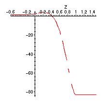
> display([pbkN41,pbkN42,pbkN43]);

Here the plot is significantly better, and we find that if we evaluate the function at a point between z=0 and L we get a real number.

> Z:=.5;Theta2bk;

If we evaluate the Maple solution at this point, we find almost the same answer only with a small imaginary term. This is probably due to round off error in the course of working the problem.

> PlotN42;

Maple cannot plot the function with such a small round off error, however it can be done in Matlab and the results are shown on the main page of the report. The imaginary term is so small that it can be neglected.The Matlab plot is done ignoring the imaginary term.

>