Figure 1
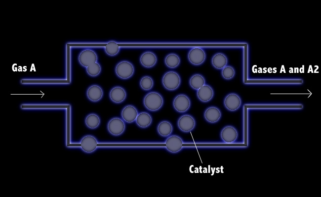
Example 17.3-1. Diffusion with Slow Heterogeneous Reaction
Problem: Consider a catalytic reactor in which the reaction gas A is converted to A2 (see Figure 1). The rate at which A disappears at the catalyst-coated surface is proportional to the concentration of A at that surface:
Figure 1
Solution: (computed on Maple V)
> restart;
Define the law of diffusion (Eq 17.0-1).
> deq:=NAz=-c*DAA2*diff(xA(z),z)+xA(z)*(NAz+NA2z);
![]()
Using stoichiometry, NA2z can be defined in terms of NAz.
> NA2z:=-1/2*NAz;
![]()
The stoichiometry of the reaction plus the law of diffusion leads to an expression for NAz in terms of the concentration gradient.
> NAza:=solve(deq,NAz);
![[Maple Math]](images/ex17_3_13.gif)
This is equivalent to Eq. 17.3-2.
For ideal gas mixtures at constant temperature and pressure, c is a constant, and DAA2 can be considered independent of concentration. -c*DAA2 can be taken outside of the derivative to get
> constNAz:=-NAza/(c*DAA2);
![[Maple Math]](images/ex17_3_14.gif)
A mass balance on species A over a thin slab of the gas film of thickness delta z leads to the equation
> ddeq:=diff(constNAz,z);
![[Maple Math]](images/ex17_3_15.gif)
The second-order differential equation is solved using the two boundary conditions: (1) at z=0, xA=xA0 and (2) at z=delta, xA=NAz/(c*k1"). (k1"=k1pp)
> s:=dsolve({ddeq,xA(0)=xA0,xA(delta)=NAz/c/k1pp},xA(z));
![]()
![[Maple Math]](images/ex17_3_17.gif)
> assign(s); xA:=unapply(xA(z),z);
![[Maple Math]](images/ex17_3_18.gif)
BS&L solves for (1-1/2*xA). To check this solution, the same computation can be carried out and compared. Unfortunately a good deal of simplification has to be done by hand to compare the two, as Maple is too stubborn Tto do it in a few easy steps.
> simplify(%,assume=positive);
![[Maple Math]](images/ex17_3_19.gif)
(See, it doesn't work.)
> a:=1-1/2*xA(z);
![[Maple Math]](images/ex17_3_110.gif)
> b:=simplify(a);
![[Maple Math]](images/ex17_3_111.gif)
This is where the ugliness begins. I begin by expanding the exponential term into two. This computation automatically gets rid of some of the natural log terms that Maple should have canceled itself.
> b:=-1/2*delta*(exp(z/delta*ln(-(2*c*k1pp-NAz)/(c*k1pp*(-2+xA0))))*exp(ln(1/delta*(ln(-(2*c*k1pp-NAz)/(c*k1pp*(-2+xA0)))*(-2+xA0)))))/ln(-(2*c*k1pp-NAz)/(c*k1pp*(-2+xA0)));
![[Maple Math]](images/ex17_3_112.gif)
Again I have to manually get rid of the exp(ln(...)).
> b:=-1/2*(-(2*c*k1pp-NAz)/(c*k1pp*(-2+xA0)))^(z/delta)*(-2+xA0);
![[Maple Math]](images/ex17_3_113.gif)
From now on it's just rearranging of terms.
> b:=subs((-(2*c*k1pp-NAz)/(c*k1pp*(-2+xA0)))^(z/delta)=(-1)^(z/delta)*((2*c*k1pp-NAz)/(c*k1pp*(-2+xA0)))^(z/delta),%);
![[Maple Math]](images/ex17_3_114.gif)
> b:=subs(((2*c*k1pp-NAz)/(c*k1pp*(-2+xA0)))^(z/delta)=(1-1/2*NAz/(c*k1pp))^(z/delta)*2^(z/delta)*(-2+xA0)^(-z/delta),%);
![[Maple Math]](images/ex17_3_115.gif)
> b:=subs({(-1)^(z/delta)*2^(z/delta)*(-2+xA0)^(-z/delta)=(1-1/2*xA0)^(-z/delta),-1/2*(-2+xA0)=(1-1/2*xA0)},%);
![[Maple Math]](images/ex17_3_116.gif)
Maple will no longer substitute/simplify terms for some reason. After more simplification, 1-1/2*xA becomes
> b:=(1-1/2*NAz/(c*k1pp))^(z/delta)*(1-1/2*xA0)^(1-z/delta);
![[Maple Math]](images/ex17_3_117.gif)
This is equivalent to Eq. 17.3-12.
NAz can be calculated at z=0.
> NAzb:=solve(deq,NAz);
![[Maple Math]](images/ex17_3_118.gif)
![[Maple Math]](images/ex17_3_119.gif)
And it's our wonderful friend LambertW. To check the answer (the local rate of conversion from A to A2), compare this solution to Eq. 17.3-13.
> bookeq:=NAz=2*c*DAA2/delta*ln((1-1/2*NAz/(c*k1pp))/(1-1/2*xA0));
![[Maple Math]](images/ex17_3_120.gif)
> bookNAz:=solve(bookeq,NAz);
![[Maple Math]](images/ex17_3_121.gif)
![[Maple Math]](images/ex17_3_122.gif)
> NAzb-bookNAz;
![]()
Yes!
So the answer attained via Maple is correct.
Because the equation for NAz is transcendental, BS&L attempts to simplify the equation by expanding ln(1-1/2*NAz/(c*k1pp)) into a Taylor series when k1pp is large and discarding all the terms but the first. I, too, will attempt to do the same.
The dimensionless group DAA2/k1pp/delta is convenient in converting NAzb into a function of x.
> k1pp:=DAA2/x/delta;
![]()
> NAzbtaylor:=taylor(1/NAzb,x=0,2);
Error, (in series/fracpower) unable to compute seriesMaple V will not allow me to use this command with the LambertW function, but it worked with the older version of Maple. :(
Since Maple will not compute the Taylor series expansion, any methods now will not be of much help when trying to compare with the Taylor solution in the book.
But I will try anyway and see what happens. I plan to compare the plots of my solution (without the Taylor series expansion) and BS&L's solution (with the Taylor series expansion). First I define NAzb and the book's answer as functions of x.
> NAzc:=x->-2*exp(-(LambertW(-1/2*(-2+xA0)*exp(1/x)/x)*DAA2-DAA2/x)/DAA2)*c*DAA2/(x*delta)+exp(-(LambertW(-1/2*(-2+xA0)*exp(1/x)/x)*DAA2-DAA2/x)/DAA2)*c*DAA2*xA0/(x*delta)+2*c*DAA2/(x*delta);
![[Maple Math]](images/ex17_3_125.gif)
![[Maple Math]](images/ex17_3_126.gif)
> NAztaylor:=x->2*c*DAA2/delta/(1+DAA2/k1pp/delta)*ln(1/(1-1/2*xA0));
![[Maple Math]](images/ex17_3_127.gif)
> k1pp:=DAA2/x/delta; NAztaylor(x);
![]()
![[Maple Math]](images/ex17_3_129.gif)
To plot, the parameters need to be defined numerically. The composition of A at the edge of the gas film is 0.95. The diffusivity is 1.26E-5 cm2/sec. The catalytic surface is 0.01 cm from the edge of the film. The molar concentration is 1 mol/cm3.
> xA0:=0.95; DAA2:=1.26E-5; delta:=0.01; c:=1;
![]()
![]()
![]()
![]()
> plot({NAzc(x),NAztaylor(x)},x=0...1000);
> plot(NAzc(x)-NAztaylor(x),x=0...1000);
Obviously, the two plots are not the same. The discrepancy arises from the fact that my solution plots the whole entire function while BS&L's solution is only the first term of a Taylor series expansion of the solution.
RECOMMENDATION: Do this problem by hand. The integration takes a lot less time and effort and results in an answer that's comparable to BSL's solution.