> restart;

Our first duty will be to apply the Stefan-Maxwell equations to our situation. For this problem, we will represent component A by indices 1, B by indices 2, and An by indices 3. Also, since B is stagnant, its flux (N[B]) is zero. Another assumption is that D[ij]=D[ji].

> N[2]:=0;Dbinary[1,2]:=Dbinary[2,1];Dbinary[1,3]:=Dbinary[3,1];Dbinary[2,3]:=Dbinary[3,2];

The next part will be to start with the Stefan-Maxwell equation on page 570 (18.4-19) Here, the length of the z interval is delta. We are deriving equations for component A and B, or 1 and 2. Below is the differentiation of x[i] with resect to z.

> stefanleftA:=diff(x[1](z),z)/delta;stefanleftB:=diff(x[2](z),z)/delta;

The right side of the equations show how x varies with the diffusivity:

> stefanrightA:=sum((x[1](z)*N[j]-x[j](z)*N[1])/(c*Dbinary[1,j]),j=1...3);

> stefanrightB:=sum((x[2](z)*N[j]-x[j](z)*N[2])/(c*Dbinary[2,j]),j=1...3);

Now we will set the two sides equal to each other:

> eq1:=stefanleftA=stefanrightA;

> eq2:=stefanleftB=stefanrightB;

We will first simplify the eq2, which deals with x[B]. Multiplying both sides by c*Dbinary[An,B]:

> eq2:=(%*c*Dbinary[3,2]);

Another simplification can be made, knowing that N[Az]=-n*N[Anz].

> N[3]:=(-1/n)*N[1];deltax[B]:=simplify(eq2);

Finally, by dividing both sides by N[1]:

> eq2:=(%/N[1]);

Since v[AnB]=N[1]*delta/(c*Dbinary[AnB]), and r[B]=D[AnB]/D[AB], then the above equation agrees with the book!

> Dbinary[2,1]:=Dbinary[3,2]/r[B];N[1]:=v[AnB]*c*Dbinary[3,2]/delta;simplify(eq2);

THE ABOVE EQUATION AGREES WITH 18.5-30 IN THE BOOK! We will now work on deriving 18.5-29:

We must first see how eq1 appears with the simplifications we have already introduced:

> eq1;

We will now define r[An], using the definition given in the book:

> Dbinary[3,1]:=Dbinary[3,2]/r[An];

> simplify(eq1);

This looks very similar to eq. 18.5-29 in the book. If we can just bring over the v[AnB] term and cancel out the extra delta:

> eq1:=simplify(eq1*delta/v[AnB]);

Finally, we note that x[1]+x[2]+x[3]=1, since all mole fractions must add up to one:

> x[3]:=1-x[2]-x[1];

> eq1:=simplify(eq1);

THIS IS THE EXPANDED FORM OF EQUATION 18.5-29 in the book. We have derived the Stefan-Maxwell equations for this problem!

Now, we will begin solving for the mol fractions of components A and B. Once again, we will begin with component B:

> eq2left:=1/x[2];eq2right:=(r[B]-1/n)*v[AnB]; Equation 18.5-30

We will define the constant R as in the book:

> r[B]:=R+1/n;

Now we will separate variables to prepare for integration.

> find1:=int(eq2left,x[2]=x2o...x2)=int(eq2right,epsilon=0...epsilon1);

By solving for x[2] we find:

> x2:=solve(%,x2);

THIS IS EQUATION 18.5-31 in the book. We will now subsititute this into Eq. 18.5-29 and solve for x[A]. To solve for x[A], we begin by defining the right and left sides of the equation equivalent to 18.5-29 that we found earlier:

> eq1left:=1/x[1];

> eq1right:=v[AnB]*(-x[2]*r[B]*n-r[An]*x[1]-r[An]*n+r[An]*n*x[2]+r[An]*n*x[1])/(n*x[1]);

Redefining x[2] to correct for notation, and setting the left and right sides equal:

> x[2]:=x2;eq1right;

> find2:=int(eq1left,x[1]=x1o...x1)=int(eq1right,epsilon1=0...epsilon);

Now, we will solve the above expression for x[1], or the mole fraction of component A:

> x[1]:=x1;xA:=solve(find2,x[1]); THIS IS OUR SOLUTION FOR x[A]:

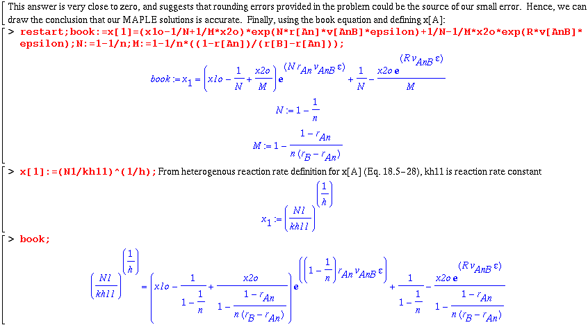
> book:=(x1o-1/N+1/M*x2o)*exp(N*r[An]*v[AnB]*epsilon)+1/N-1/M*x2o*exp(R*v[AnB]*epsilon);

> N:=1-1/n;M:=1-1/n*((1-r[An])/(r[B]-r[An]));

> book; Eq 18.5-32 in Book

Admittedly, our expression is an unpleasant solution involving a complicated intrinsic MAPLE function known as LambertW. In addition, taking the difference between this solution and the book's equation (18.5-32) gives a long, messy answer. Hence, I will try to show the validity of our MAPLE solution with an example.

This problem entails a gas component, Air, diffusing through a stagnant film to reach the Carbon, which is involved in a combustion reaction to form Carbon Dioxide. The carbon particle is a sphere. The reaction can be written as:

Several assumptions and data are provided in the problem:

• The Nitrogen is not involved in the reaction, and is taken to be stagnant.
• The Oxygen is the "diffusing gas."
• The Carbon is considered the catalyzing surface.
• The Oxygen and Carbon react in a 1 to 1 ratio, so that n=1.
• The reaction is heterogeneous.
• The radius of the particle is 0.0254 cm.
• The concentration can be taken as an ideal gas:c=(n/V)=P/RT
• The pressure is standard bar, the temperature is 1366.67 K
• Ratio of diffusivities are: (CO2-N2/CO2-O2)=0.91356, (CO2-N2)/(N2-O2)=0.80097.
• N[O2]=0.84 lbmol/(hr*ft^2), D[O2,N2]=6 ft^2/hr.

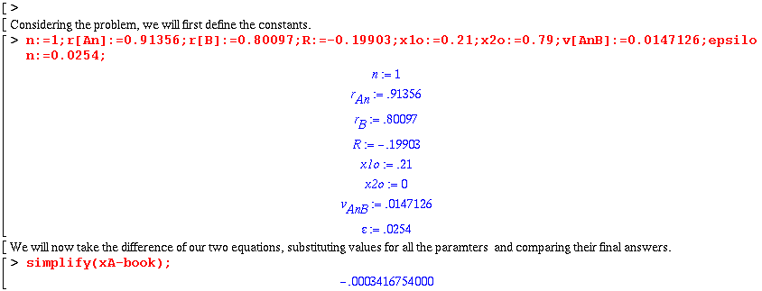
We will now use the data taken from the example problem and sources to see if the derived MAPLE solution for x[A] is equivalent to the book. Note that component A=1=O2, B=2=N2, An=3=CO2.