Example 9.6-1 Composite Cylindrical Walls

Bird,Stewart, and Lightfoot pg.286

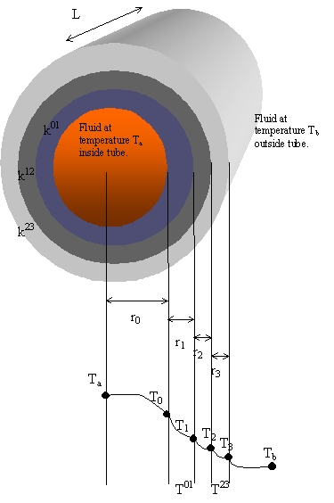
     This problem deals with conduction through a composite cylindrical wall made up of three different layers, with three separate thicknesses and thermal conductivities.  This example is an extension of the main example in section 9.6 which deals with a recta linear system.  The diagram below illustrates a fluid within a cylinder at temperature Ta that is transferring heat across a composite cylinder wall to a cooler fluid at temperature Tb outside the cylinder.  The goal of this problem is to combine the different resistances of the layers into one total resistance.

     In order to find the combined resistance of the three layers, one must first compute the resistance of each individual layer.  The layers are of thickness (r₁-r₀), (r₂-r₁), and (r₂-r₃) and have thermal conductivities k¹⁰, k¹², k²³.  The first layer, "01" is in direct contact with the fluid inside the cylinder at temperature T_a, and the outermost layer "23" is in direct contact with the surrounding fluid at T_b.  The heat flux is known to be at steady state, and Newton's "law of cooling" applies at the fluid-solid interfaces at r=r₀ and r=r₃.  The process of finding the individual resistances and combining them into an overall resistance is shown in the following Maple session.

> restart;

First solve a the generic differential equations for one shell, then generalize it and compute the equations for every shell. Label the inside conditions "A" and the outside conditions "B" for ANY shell.

Fourier's Law of Heat Conduction

> q:=(r,k)->-k*D(T)(r);

Thermal Energy Balance for a cylindrical shell of volume 2**r*L*r

> SurfArea:=r->2*Pi*r*L;

> Q:=(r,k)->q(r,k)*SurfArea(r);

> balance:=Q(r,k)-Q(r+dr,k)=0;

Divide the energy balance by 2**L*k*r and take the limit as r approaches 0.

> deq:=limit(lhs(balance)/(2*Pi*L*k*dr),dr=0)=0;

Solve the differential equation with the known temperatures on the inside wall, and outside wall.

> s:=dsolve({deq,T(rA)=TA,T(rB)=TB},T(r));

> assign(s);T:=unapply(T(r),r);

Plug the results into the formula for the heat flux, and solve for Ta-Tb.

> q(r,k);

Because the system is in steady state and not accumulating any heat, the total flux through every wall is constant. This constant flux can be called 2**r0*L*q0, which is the flux at the inner wall.  Since both terms contain 2**L,  r*q is the same for all surfaces.

> geneqn:=q(r,kab)*r=q0*r0;

> gensoln:=TA-TB=solve(geneqn,(TA-TB));

Generalize the equation, for each of the 3 layers.

> T:=array(0..3,[]): r:=array(0..3,[]):

> eqs:=array(0..4,[]): ks:=array(0..3,0..3,[]):

> for j from 0 to 2 do

> eqs[j+1]:=T[j]-T[j+1]=r[0]*q0*(ln(r[j+1])-ln(r[j]))*1/ks[j,(j+1)];

> od;

Equations 9.6-24 through 9.6-26 are produced.

Next, Newton's Law of cooling is used to find relationships between the two fluid-solid interfaces. Here "a" and"b" are not longer generic descriptors. "a" represents the conditions inside the tube, and "b" represents the conditions outside the tube.

> eqs[0]:=Ta-T[0]=q0/h0;

To find the heat flux at the outer wall in terms of q0, we again use the steady state condition.

> stdystate:=q3*2*Pi*r[3]*L=q0*2*Pi*r[0]*L;

> q3:=solve(stdystate,q3);

> eqs[4]:=T[3]-Tb=q3/h3;

Sum all five equations to get a result in terms of the known temperatures Ta and Tb.

> sumeqns:=sum(eqs[k],k=0..4);

Now, q0 and Q0 can be solved for in terms of our two known temperatures.

> q0:=solve(sumeqns,q0);

> Q0:=SurfArea(r[0])*q0;

The "overall heat transfer coefficient based on the inner surface" called U0 is computed. Unlike a
recta linear system, the overall heat transfer coefficient must be based on the surface of one of the
layers. This is because the surface are of each consecutive layer is larger than the previous, and
conversely the relative heat flux q, becomes smaller.

> U0:=(Q0/((Ta-Tb)*SurfArea(r[0])));

The reciprocal of U0 looks very similar to the reciprocal of U0 shown in the book if the log terms are combined.

> solution:=expand(1/U0);

The answer is checked with the book, and, after some simplification, is found to agree.

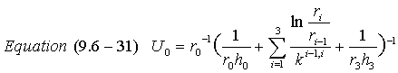
> U0book:= r[0]^(-1)*( (1/(r[0]*h0)+sum(ln(r[i+1]/r[i])/ks[i,(i+1)],i=0..2)+(1/(r[3]*h3))) )^(-1);

Help Maple simplify by expanding the ln terms in the books answer.

> for n from 0 to 2 do

> U0book:=algsubs(ln(r[n+1]/r[n])=ln(r[n+1])-ln(r[n]),U0book):

> od:

> simplify(U0-U0book);

Re-enter the formula for U0 (use books form)

> U0:= r[0]^(-1)*( (1/(r[0]*h0)+sum(ln(r[i+1]/r[i])/ks[i,(i+1)],i=0..2)+(1/(r[3]*h3))) )^(-1);

Assume a 1 ft. diameter pipe is surrounded by 1/2 inch of cork which is then surrounded by
1/2 inch of a brick like material.

Inner radius and thermal conductivity of a 1 ft diameter steel pipe

> r[0]:=.5*ft; ks[0,1]:=26.1*Btu/(hr*ft*F);

Inner radius and thermal conductivity of 1/2 inch cork layer

> r[1]:=r[0]+.5*ft; ks[1,2]:=.03*Btu/(hr*ft*F);

Inner radius and thermal conductivity of the 1/2 inch insulating brick layer

> r[2]:=r[1]+.5*ft; ks[2,3]:=.9*Btu/(hr*ft*F);

Outer radius of the insulating brick layer

> r[3]:=r[2]+.5*ft;

Assume a liquid in the pipe, and air around the pipe. Reasonable heat transfer coefficients are chosen.

> h0:=200*Btu/(hr*ft^2*F); h3:=120*Btu/(hr*ft^2*F);

Assume the liquid is at 200 F and the air is at 60 F

> Ta:=200*F; Tb:=60*F;

This is the "over-all heat transfer coefficient"

> U0;

Note:
 

The general equation for U0, eq. 9.6-31, is found by observing the pattern in U0 for this problem and noting that ln terms in the denominator are the ln of the outer radius over the inner radius all over the heat transfer coefficient for the layer.  Additionally, the final term in the denominator is the reciprocal of the outermost radius multiplied by the outer heat transfer coefficient.  See pg. 288 for a discussion of this.