In order to do this problem we must make the following assumptions:

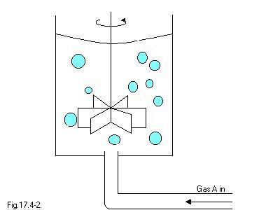
a.) Each gas bubble is surrounded by a stagnant liquid film of thickness delta, which is small with respect to the bubble diameter.

b) A steady-state concentration is quickly established in the liquid film after the bubble if formed.

c) The gas A is only sparingly soluble in the liquid, so that we can neglect the bulk flow term in Eq. 17.0-1.

d) The bulk of the liquid outside the stagnant film is at concentration c_{A delta}, which changes so slowly with respect to time that it can be considered to be constant.

Eq. 17.0-1;

> N[Az]:=-c*D[AB]*diff(x[A](z),z)+x[A]*(N[AZ]+N[Bz]);

Is now reduced to

> N[Az]:=z->-DAB*D(cA)(z);

By performing a mass balance through a differential segment z we get :

> eq:=-limit((N[Az](z)-N[Az](z+dz))/dz,dz=0)+k1*cA(z)=0;

Now we apply the boundary conditions and solve for c_A(z);

B.C. 1 at z = 0, =

B.C. 2 at z =

> s:=dsolve({eq,cA(0)=cA0,cA(delta)=cAdelta},cA(z)); Finding a solution for Ca and making Ca a function of z

> assign(s);cA:=unapply(cA(z),z);

 

Next we change our variables to simplify our expressions, and make c_A a function of zeta;

> z:=zeta*delta;cAdelta:=cA0*Gamma;k1:=b1^2*DAB/delta^2;assume(b1>0);assume(delta>0);assume(zeta>0); Changing variables to make expressions look less complicated

 > C[A]:=zeta->simplify(convert(cA(z),trig)); It's more convenient to have Ca as a function of instead of z

> C[A](zeta);

In the case of no chemical reaction;

> eq13:=(c[A]/cA0)=limit(C[A](zeta)/cA0,b1=0): I took the limit because substituting 0 for b1 gives a division by zero error.

> solve(eq13,{c[A]/cA0});

The mass fluxes for absorption with and without reaction are;

> N[Az]='N[Az]': I had to define as a variable, since I already used it at the beginning, so that I could redefine it here

> k:=(-DAB*diff(C[A](zeta),zeta))/delta; This is Eq. 17.4-14. I divided it by delta because I'm taking the derivative with respect t . According to the chain rule d(Ca) /d z = d(Ca)/d * d /dz

> N[Az]:=unapply(k,zeta); Making a function of

> N[Az](0); Setting = 0, because z = 0, to obtain Eq.17.4-14

> c[A]:=solve(eq13,c[A]); Obtaining from eq13, which is a few lines above

> N[Aznorxn]:=(-DAB*diff(c[A],zeta))/delta; Eq. 17.4-15

To obtain eq 17.4-16;

> Gamma:=0:N[Aznorxn]; =0 in eq. (17.4-15) but not in eq. (17.4-14)

> Gamma:='Gamma': Defining as a variable, so that the previous definition of doesn't affect the in Eq.17.4-14

> Nstr:=N[Az](0)/(DAB*cA0/delta); Eq. 17.4-16

To obtain eq. (17.4-18) we must evaluate d /dz at z = and, because of B.C. 2, set eq. (17.4-12) equal to

> eq2:=C[A](zeta)=cAdelta; Substituting cAdelta for cA in Eq. 17.4-12

> Cad:=solve(eq2,cAdelta); I defined cAdelta as cA0 above, so this command just solves eq2 for cA0 , a quanitty that I chose to call Cad

Next we must equate the mass of A crossing the outer surface of the film with the amount of A being removed by chemical reaction in the bulk of the liquid;

> eq3:=-A*DAB*(diff(Cad,zeta)/delta)=V*k1*cAdelta; Eq. (17.4-17)

> funct:=unapply(eq3,zeta); Changing eq3 to funct( ) so that I can evaluate it at = 1

> funct(1); at z = , = 1

> gama:=solve(funct(1),Gamma); Eq. 17.4-18

> Gamma:=gama; Using the above solution to define

> fnleq:=simplify(Nstr); Eq.17.4-19

 

In order to create the plot of N* vs. b1 I used the books expression for Eq. 17.4-19, because Maple would not rearrange my expression so that I could substitute different values for V/Adelta.

> restart;

> Nbk:=(b1/sinh(b1))*(cosh(b1)-1/(cosh(b1)+b1*(alpha)*sinh(b1))); I substituted alpha for (V/Adelta)

> alpha:=0:

> p1:=loglogplot(Nbk,b1=.1e-3..10,y=.8..1.5): This command just saves a bunch of numbers in p1, that are displayed later on

> alpha:=10^2:

> p2:=loglogplot(Nbk,b1=.1e-3..10,y=.8..1.5):

> alpha:=10^4:

> p3:=loglogplot(Nbk,b1=.1e-3..10,y=.8..1.5):

> alpha:=10^6:

> p4:=loglogplot(Nbk,b1=.1e-3..10,y=.8..1.5):

> alpha:=10^8:

> p5:=loglogplot(Nbk,b1=.1e-3..10,y=.8..1.5):

> alpha:=10^100:

> p6:=loglogplot(Nbk,b1=.1e-3..10,y=.8..1.5):

> with('plots'): This allows you to make log-log plots and do about a million other cool things with graphs

> display([p1,p2,p3,p4,p5,p6]);

This plot does is almost like the one in the book except for the seemingly straight lines. I think that the lines are not as curvy because I made the plot on log-log scale.

Find the ratio of the absorption rate with a first-order reaction to the absorption rate with a zero order reaction, i.e. no reaction, using the following data:

V = 100 m^3, A = 1 m^2, delta = 1 m

> restart;

>Nstar:=(b1*(b1*sinh(b1)*cosh(b1)*V+A*delta*(cosh(b1))^2A*delta))/(A*sinh(b1)*delta*cosh(b1)+V*b1*(cosh(b1))^2-V*b1);

> b1:=.8;V:=100;delta:=1;A:=1;

> Nstar;