Example 11.2-2. Laminar Tube Flow with Constant Heat Flux at Wall: Asymptotic Solution for Small Distances

By Susan Ireland and Drew Vennum

This is a continuation of example 11.2-1 developing an expression for T(r,z) that is useful for small z values.
Because z is small, heat diffuses only into a very small layer near the inside edge of the tube. This means the tube can be treated like a flat wall of width Pi*diameter, and leads to the assumptions that:
a. Distance from the wall is s = R - r.
b. Fluid may be taken to extend from s = 0 to s = infinity
c. Velocity profile is linear because the effects from the opposite wall of the pipe are not felt. This leads to the velocity profile:
v_z(s) = v_os/R, where v_o = (p_o - p_L)R²/2mL

> restart;

> vz:=s->v0*s/R; Declare velocity profile as a function of s

> eq10:=vz(s)*diff(T(s,z),z)=alpha*diff(diff(T(s,z),s),s); Energy equation: 11.2-10

[Maple Math]

We convert this formula by substituting q_s for T, where . This is done by dividing both sides by s, then differentiating both sides with respect to s.
> eq10:=eq10/s:

> de:=diff(eq10,s);

[Maple Math]

> de:=subs(diff(T(s,z),s)=qs(s,z)/k,de):

> de:=simplify(de*k); This is Eq. 11.2-11

[Maple Math]

We will convert to dimensionless variables:
, ,

> with(PDEtools,dchange); transf:={qs(s,z)=psi*q1,s=eta*R,z=lambda*v0*R^2/alpha}:

> Newde:=dchange(transf,de,[psi(eta,lambda),(eta,lambda)]):

> eq13:=simplify(%*R^3/(alpha*q1)); Eqn. 11.2-13

[Maple Math]

> eqbook:=simplify(diff(psi(eta,lambda),lambda)=diff(1/eta*(diff(psi(eta,lambda),eta)),eta)): simplify(eq13-eqbook);

This shows that the Maple eq13 is actually BS&L's Eq. 11.2-13
The boundary conditions for these variables are:
Boundary Conditions:
at

We will now use the method of combination of variables to replace with where

It can easily be verified that this still fits the boundary conditions of the problem.

The following steps convert the LHS of Eq 11.2-13 using the relation
> equiv:=diff(psi(chi),chi)=diff(psi(eta,lambda),lambda)*diff(lambda(chi),chi);

> eq17:=chi=eta/(9*lambda)^(1/3);

[Maple Math]

> solve(eq17,lambda);

> lambda:=chi->eta^3/9/chi^3:

> LHS:=diff(psi(chi),chi)/diff(lambda(chi),chi);

[Maple Math]

Now we convert the RHS using the relation .
> equiv2:=diff(1/eta*diff(psi(eta,lambda),eta),eta)=diff(chi(eta),eta)*diff(1/eta*diff(psi(chi),chi)*diff(chi(eta),eta),chi);

[Maple Math]

> solve(eq17,eta);

[Maple Math]

> chi:=eta->eta/(9*lambda)^(1/3):

> eta:=chi->chi*(lambda*9)^(1/3):

> RHS:=diff(chi(eta),eta)*diff(1/eta(chi)*diff(psi(chi),chi)*diff(chi(eta),eta),chi);

[Maple Math]

We combine the LHS and RHS to give an ordinary differential equation in c.
> eq18:=simplify(LHS-RHS);

[Maple Math]

We then simplify by substituting to replace all instances of the old variables with the new variable
> eq18:=subs(eta=chi*(9*lambda)^(1/3),eq18);

[Maple Math]

By simplifying and multiplying both sides by common factors, we obtain:
> ode:=simplify(eq18*(-9)*chi^2*lambda); Eqn. 11.2-18

[Maple Math]

Unfortunately, Maple does not know the solution to this problem
> sol:=dsolve({ode,psi(0)=1, psi(infinity)=0},psi(chi));

Error, (in dsolve/sysODE) dsolve/sysODE expects its 2nd argument, funcs, to be of type {set({name, Function}), list({name, Function})}, but received psi(chi)

This has to be solved another way. We converted the second order equation to a system of first order equations by substituting .
> ode1:=3*chi^3*pi(chi)-pi(chi)+chi*diff(pi(chi),chi);

We rewrite Eq 11.2-18 in terms of Pi. We separated the variables to different sides of the equation and integrated each side.
> eq:=3*chi^3*pi-pi+chi*dpi/dchi=0;

> solve(eq,pi);

[Maple Math]

> LHS:=int(-1/pi,pi);

> RHS:=int((3*chi^3-1)/chi,chi);

We combine them and add the constant of integration.
> eq:=LHS=RHS+c1;

We solve this for pi, which is actually y'.
> de:=solve(eq,pi);

We then integrate this to find y(c). As you can see, Maple has decided to grace us with its famous WhittakerM functions
> psi:=int(de,chi);

[Maple Math]

> simplify(psi,assume=positive);

[Maple Math]

We simplify, declare y(c) as an actual function, and add the second constant of integration.
> psi:=chi->1/10*exp(-1/2*chi^3-c1)*(2*WhittakerM(1/3,5/6,chi^3)+3*WhittakerM(-2/3,5/6,chi^3))/(chi^2)+c2;

[Maple Math]

We attempt to use the boundary conditions to solve for the constants. The boundary conditions are:
a)

and
b)

First apply B.C. b)
> eqa:=0=psi(infinity);

[Maple Math]

This equation has 0/infinity +c2 =0, so it is obvious that:
> c2:=0;

Again Maple has problems with the solution and cannot evaluate y(0).
> psi(0);

Error, (in psi) division by zero

We try to solve for c1, but Maple returns no output.
> solve(psi(chi),c1);

At this point we check the BS&L solution Eq 11.2-19 to show that it satisfies the differential equation 11.2-18
> psi:=chi->Int(chi1*exp(-chi1^3),chi1=chi...infinity)/Int(chi1*exp(-chi1^3),chi1=0...infinity);

[Maple Math]

> d1psi:=diff(psi(chi),chi);

[Maple Math]

> d2psi:=diff(diff(psi(chi),chi),chi);

[Maple Math]

> chi*d2psi+(3*chi^3-1)*d1psi;

[Maple Math]

The above equation is the LHS of equation 11.2-18, and it should simplify to 0
> simplify(%);

At this point we do some nifty calculations outside of Maple to show how the final solution is obtained.

We start by integrating Fourier's Law to obtain the temperature profile:

we convert to dimensionless quantities using the following substitutions for change of variables:
, so:
and

We know from the previous conversion to dimensionless form that .
With a little algebra we obtain Eq 11.2-21, which is:

Substitution of the BS&L solution for y(c) gives:

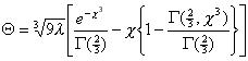
Where is the "complete gamma function" and is the "incomplete gamma function"
The solution for y(c) is analagous to 1 - erf, but the coefficient on p is (3c - 1) rather than 2c. Because it takes this form, it is not at all surprising that Maple is unable to solve our ODE when it easily solves differential equations whose solutions involve the common error function.