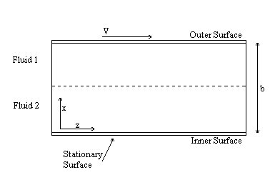
In BSL 2.5, the velocity profile for two immiscible fluids flowing due to a pressure drop (Poiseuille) was calculated. However, BSL does not address Couette flow for this system, and the temperature profile is never analyzed in later chapters. This oversight is corrected with our Maple project, which not only solves for the velocity and temperature distributions for a system of two immiscible fluids between flat plates, but also graphs the profiles using representative values to show the effect of changing each variable.

> restart;

> eq1:=diff(tau1(x),x)=0; eq2:=diff(tau2(x),x)=0;

The Shear Stress (Tau) is constant throughout each Fluid.

1 refers to Fluid 1 - The fluid that is in contact with the moving plate

2 refers to Fluid 2 - The fluid that is in contact with the stationary plate

> eq3:=dsolve({eq1,tau1(b/2)=(V-Vzmid)*2*mu1/b},tau1(x)); assign(eq3): tau1:=unapply(tau1(x),x): eq4:=dsolve({eq2,tau2(b/2)=(V-Vzmid)*2*mu1/b},tau2(x)); assign(eq4): tau2:=unapply(tau2(x),x):

The boundary conditions are set by the equation, Tau = diff(vz,x)*mu (Eqn 2.2-12 pg 39). The differential, diff(vz,x) can be approximated with

diff(vz,x) = (V-Vzmid)/(b/2) where b = length separating the two plates

V = Velocity of moving plate

Vzmid = Velocity at contact point of fluid (at b/2)

> eq5:=tau1(x)=diff(vz1(x),x)*mu1; eq6:=tau2(x)=diff(vz2(x),x)*mu2;

Egn 2.2-12 (pg 39)

> s:=dsolve({eq5,vz1(b)=V},vz1(x)): assign(s); s:=dsolve({eq6,vz2(0)=0},vz2(x)): assign(s); vz1:=unapply(vz1(x),x); vz2:=unapply(vz2(x),x);

The bounday conditions are set by our initial conditions.

B.C.1 @ x = b, vz1 = V

B.C.2 @ x = 0, vz2 = 0

> eq7:=Vzmid=simplify(vz2(b/2));

Use the condition where @ x = b/2 vz2 = Vzmid

> Vzmid:=solve(eq7,Vzmid);

Solves for Vzmid in terms of the viscosities of Fluid 1 and Fluid 2 and V

> vz1(x); vz2(x);

Now we have equations for vz1 and vz2 in terms of the viscosities, the length (b), and V.

> Sv1:=mu1*diff(vz1(x),x)^2; Sv2:=mu2*diff(vz2(x),x)^2;

The viscous heat source (Sv) is defined by Sv = mu*(diff(vz,x))^2 (Eqn 9.4-1 pg 277)

> Qx1:=x->W*L*qx1(x); Qx2:=x->W*L*qx2(x);

Total heat movement through the two fluids in the x direction (Eqn. 9.2-16 pg 270)

> eq5:=Qx1(x)-Qx1(x+dx)+Sv1*W*L*dx; eq6:=Qx2(x)-Qx2(x+dx)+Sv2*W*L*dx;

Heat balance in each liquid, In-Out+Produced=0 at steady state (Eqn 9.1-1 pg 266)

> de1:=simplify(eq5/(W*dx*L)); de2:=simplify(eq6/(W*dx*L));

Divide each side of the equations by the differential volume

> de3:=limit(de1,dx=0); de4:=limit(de2,dx=0);

Take the limit as dx->0 to give differentials in place of the deltas, definition of a derivative

> de5:=dsolve({de3,qx1(b/2)=qxconst},qx1(x)): assign(de5); qx1:=unapply(qx1(x),x); de6:=dsolve({de4,qx2(b/2)=qxconst},qx2(x)): assign(de6); qx2:=unapply(qx2(x),x);

Solve the differential equations for the boundary conditions given by the physical setup of the problem. At the interface the heat flux must be continuous, and therefore a constant for both.

> de3:=qx1(x)=-k1*diff(T1(x),x); de4:=qx2(x)=-k2*diff(T2(x),x);

Fourier's Law of Heat Conduction (Eqn 8.1-2 pg 245)

> de5:=dsolve({de3,T1(b)=Tb},T1(x)): assign(de5); T1:=unapply(T1(x),x); de6:=dsolve({de4,T2(0)=T0},T2(x)): assign(de6); T2:=unapply(T2(x),x);

Solve the differential equtians for the given boundary conditions:

B.C.1 @x=b T1=Tb

B.C.2 @x=0 T2=T0

> eq10:=T1(b/2)=T2(b/2);

Temperature must be continuous at the interface between the two fluids

> qxconst:=solve(eq10,qxconst);

Solve for the constant heat flux term at the interface

> simplify(T1(b/2)); simplify(T2(b/2));

Show temperatures at the interface to be sure they agree

> T1(x):=simplify(T1(x)); T2(x):=simplify(T2(x));

Final temperature profile in each fluid

>

> T0:=300: Tb:=300: k1:=4e3: k2:=4e3: mu1:=20: mu2:=20: V:=100: b:=.02:with(plots):
p1:=plot([T1(x),x,x=0.01...0.02]):
p2:=plot([T2(x),x,x=0...0.01]):
display([p1,p2]);

All conditions the same for both fluids. As expected, the system is acting as a single fluid with constant properties.

> T0:=300: Tb:=310: k1:=1e3: k2:=4e3: mu1:=20: mu2:=20: V:=100: b:=.02:with(plots):
p1:=plot([T1(x),x,x=0.01...0.02]):
p2:=plot([T2(x),x,x=0...0.01]):
display([p1,p2]);

Temperature profile when liquid 1 has a lower thermal conductivity than liquid 2. Following Fourier's Law, it has a great temperature change.

> p1:=plot([vz1(x),x,x=0.01...0.02]):
p2:=plot([vz2(x),x,x=0...0.01]):
display([p1,p2]);

Following Newton's Law of Viscosity, since both liquid have the same viscosity, the velocity profile is one continuous slope.

> T0:=300: Tb:=310: k1:=4e3: k2:=4e3: mu1:=80: mu2:=10: V:=100: b:=.02:with(plots):
p1:=plot([T1(x),x,x=0.01...0.02]):
p2:=plot([T2(x),x,x=0...0.01]):
display([p1,p2]);

Temperature profile when the vicosity of fluid 1 is much higher than fluid 2.

> p1:=plot([vz1(x),x,x=0.01...0.02]):
p2:=plot([vz2(x),x,x=0...0.01]):
display([p1,p2]);

Velocity profile when viscosity of fluid 1 is much higher than fluid 2.

> T0:=300: Tb:=310: k1:=1e3: k2:=8e3: mu1:=10: mu2:=80: V:=100: b:=.02:with(plots):
p1:=plot([T1(x),x,x=0.01...0.02]):
p2:=plot([T2(x),x,x=0...0.01]):
display([p1,p2]);

Temperature profile when viscosity and thermal conductivity of fluid 2 are much higher than fluid 1

> p1:=plot([vz1(x),x,x=0.01...0.02]):
p2:=plot([vz2(x),x,x=0...0.01]):
display([p1,p2]);

Velocity profile when viscosity and thermal conductivity of fluid 2 are much higher than fluid 1.