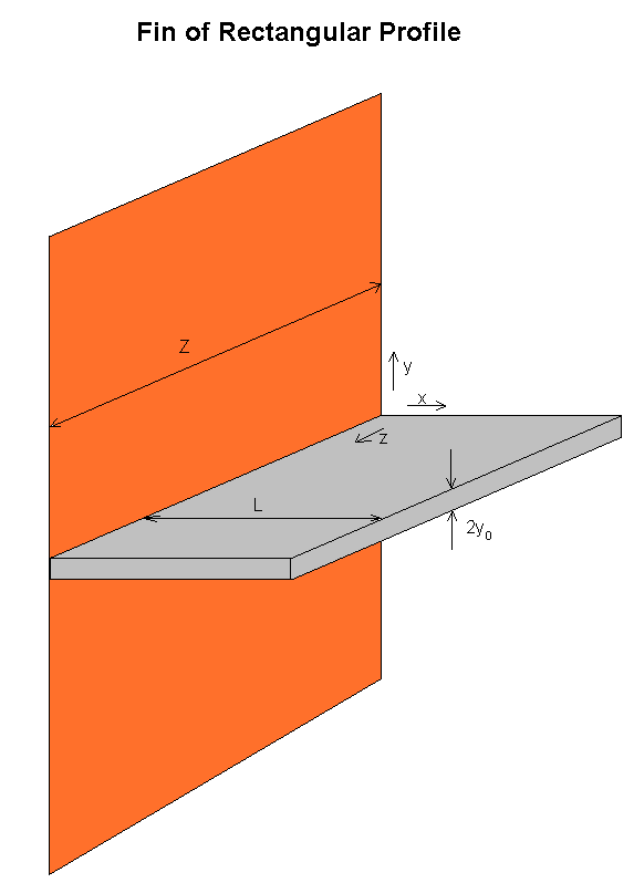
The Straight Fin of Rectangular Profile

Here we analyze the much more common case of a cooling fin. That of a rectangular profile. Since we already know the equation for the profile, we will substitute that in and see what temperature profile it generates. Lastly we will again find the characteristic Length, Height, and Area for the fin given certain conditions.

However it is important to note that the following equations will assume that no heat comes out the end. They assume that the tip of the fin is a point and as such will radiate no heat. This is obviously incorrect for a fin of this profile. So we will make the simplification that the length of the fin is NOT L, but instead is L+y0. Essentially wrapping around the edge of the fin and coming to a point. The error introduced by this is quite minimal as long as y0 is sufficiently small. Throughout this worksheet, the L represents the corrected L with the extra y0.

> restart;

Newton's Law of cooling, always a good thing to start with.

> q:=(y,x)->-k*y(x)*diff(theta(x),x);

The differential equation of the temperature distribution in fins of arbitrary profile shape.

> eqn1:=-diff(q(y,x),x)=h*theta(x):
eqn2:=simplify(eqn1/k);

General equation for total heat.

> eqn3:=qtot=h*int(theta(x),x=0...L);

General equation for Area

> eqn4:=Area=int(y(x), x=0....L);

Now we substitute the fact that our profile is linear.

> y(x):=y0;

This considerably simplifies the differential equation.

> eqn2;

Now we solve with the boundary condisions

We have reached the temperature of the environment at x=L
at x=0 the temperature of the rod is that of the heat source

> s:=dsolve({eqn2,theta(0)=theta[0],D(theta)(L)=0},theta(x)):
assign(s):
simplify(theta(x),trig);

> expand(cosh((x-L)*sqrt(h/k/y0)));

Once again, Maples simplification problems prevent us from easily converting this problem, so we will compare this to that found in the book.

> booktheta:=theta[0]*cosh((x-L)*sqrt(h/k/y0))/cosh(L*sqrt(h/k/y0));

> difference:=expand(simplify(theta(x)-booktheta));

The equation for Area, with our profile equation substituted.

> eqn4;

Now we work to simplify the qtot over Theta initial equation.

> eqn35:=simplify(convert(eqn3/theta[0],exp));

> assign(eqn35*theta[0]);

The book presents a simple equation in the form of tanh, however Maple refuses to simplify the above eqn35 to such a simple form, so we will once again show their equivalence.

> bookqtot:=theta[0]*sqrt(h*k*y0)*tanh(L*sqrt(h/k/y0));

> difference:=simplify(convert(qtot-bookqtot,exp),assume=positive);

> L:=solve(eqn4,L):

Reduce the sqrt equation inside of the tanh for simplicity. Now we will try and find what dimensions will give the maximum total heat dissipation. We will take the derivative with respect and find at what value the resulting equation goes to zero. It is at this value for u that the heat dissipation is a maximum.

> eqn5:=diff(bookqtot,y0):
eqn5:=simplify(algsubs(sqrt(h/k)*Area/y0^(3/2)=u,eqn5), assume=positive);

Now we will aim to find what value of u will make this equation equal zero. But first we need to clear some of the extra variables so we have an equation in only u.

> eqn6:=simplify(eqn5*2/theta[0]*sqrt(y0/h/k), assume=positive);

Use Maples numerical solver to find the "most favorable" value for u.

> u[f]:=fsolve(eqn6=0,u=1..3);
unassign('qtot'):

> simplify(bookqtot, assume=positive);

> unassign('k');unassign('L');
eqn7:=qtot=algsubs(sqrt(h/k)*Area/y0^(3/2)=u,bookqtot):
eqn8:=eqn7*Area*sqrt(h)/theta[0]/tanh(u)/sqrt(k*y0)/y0:
eqn9:=algsubs(Area*sqrt(h)/sqrt(k)/y0^(3/2)=u,eqn8):
k:=h/u^2*Area^2*y0^(-3):
Area:=y0*L:

Once again we generate our three characteristic equations, now for the rectangular fin.

L_eqn:=eval(solve(simplify(eqn9, assume=positive),L),u=u[f]);

> unassign('Area');unassign('k');
L:=Area/y0:
y0_eqn:=qtot=simplify(algsubs(sqrt(h/k)*Area/y0^(3/2)=u,bookqtot), assume=positive):
y0_eqn:=eval(solve(y0_eqn,y0),u=u[f]);

> Area_eqn:=L_eqn*y0_eqn;

> n:=eval(simplify(algsubs(sqrt(h/k)*Area/y0^(3/2)=u,eval(booktheta,x=L)/theta[0]), assume=positive),u=u[f]);

This last value for n here is also important to note. It says that for the most favorable ratio of width to thickness the temperature excess at the tip of the fin will be half of the temperature excess at the base of the fin next to the heat source. This n also allows us to have a quick general idea of the temperature profile throughout the fin.

Heat Conduction in the Steady State