Section 1

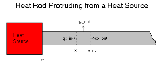
Here we generate the General Form for an equation of a heated rod.  This equation is general for rods of different cross sectional areas (and shapes).
We take the liberty of a couple simplifications which will be removed later.

> restart;

The heat flux entering a cross section is controlled by

• the cross section the heat is fluxing though

• the temperature difference across the delta X in the rod

• the heat transfer coefficient

> qx_in:=-k*SA*diff(T(x),x);

Some of this heat exits the rod vertically and is controlled by

• the surface area of the exposed rod Circumference*delx

• the temperature difference between the surface and the air

• the surface heat transfer coefficient.

> qy_out:=h*C*(T(x)-Tenv)*delx;

The third part of the heat flux is the remaining heat that isn't lost from the surface and continues through the rod.
This equation has the same parameters as the qx_in equation.

> qx_out:=-k*SA*(diff(T(x),x)+diff(T(x),x,x)*delx);

The definition of Steady State Heat Transfer, In+Out+Accumulated = 0

> SSHeatFlow:=qx_in-qx_out-qy_out=0;

> SSHeatFlow:=simplify(SSHeatFlow/delx);

Here we redefine our Temperature equation.  Instead of having it be pure temperature, it will just be the temperature difference with respect to the outside air.

> T(x):=Theta(x)+Tenv;

> SSHeatFlow:=simplify(SSHeatFlow);

Here we introduce a constant m = sqrt[( h*C)/(k*A)] for simplification.

> h:=k*m^2*SA/C;

> SSHeatFlow:=simplify(SSHeatFlow/k/SA);

> s:=dsolve(SSHeatFlow,Theta(x)):
> t:=convert(s,exp);

> simplify(t);

> GenForm:=Theta(x)=M*exp(-m*x)+N*exp(m*x);

Here these constants of integration are dependant on the boundary conditions of the system, otherwise this is the "general form" of the solution. (p208-209)
M = (C2 - C1)/2
N=(C1 + C2)/2;

Now we take the case of an "infinite rod", i.e. the length is infinite.

The Boundary Conditions.

@x = 0          Theta = Theta0
@x = infinity   Theta = 0;

> u:=dsolve({SSHeatFlow, Theta(0)=Theta[0], Theta(infinity)=0},Theta(x)):
v:=simplify(convert(u,exp),assume=positive);

Assume that we have two "very long" rods of the same shape, but different compositions, so we have: k1,k2 and h1,h2

Assume all other conditions are the same.

> assign(v);
> Theta:=unapply(Theta(x),x,m):
> eq5:=Theta(m[1],x[1])=Theta(m[2],x[2]);

Now we substitute back in for our m variable, so we can do a deeper analysis.

> unassign('h');
m[1]:=sqrt(h[1]*C/k[1]/SA);
m[2]:=sqrt(h[2]*C/k[2]/SA);

> eq6:=simplify(eq5/Theta[0],assume=positive);

Because Maple has problems simplifying equations, we'll just manually retype it in here with our simplifications.

> eq7:=x[1]*sqrt(C*h[1]/k[1]/SA)=x[2]*sqrt(C*h[2]/k[2]/SA);

> eq8:=k[1]=solve(eq7,k[1]);

Now we have two rods with the same Circumference and Cross Sectional Area.

> eq8:=simplify(eq8/k[2],assume=positive);

Thus we have a quantitative way of measuring the thermal conductivity of rods.  Knowing the thermal conductivity and the surface conductivity for two rods of equal dimensions we can find at what lengths they have the same temperature.

>

However this is a little less useful.  It would instead be easier to measure the temperature at two points of equal length on a rod, and then equate them to solve for the relationship between their surface and internal heat coefficients.

> eqn1:=Theta[1]=Theta[0]*exp(-m[1]*x);
eqn2:=Theta[2]=Theta[0]*exp(-m[2]*x);

Solve for x and substitute it into the second equation.

> x:=solve(eqn1,x);
simplify(eqn2,assume=positive);

> k[1]:=solve(eqn2,k[1]):

> eqn3:=k1/k2=k[1]/k[2];