Explanation of Free Convection and Our Problem
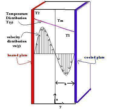
As a fluid is heated, it expands while remaining the same mass. Therefore, its density changes as it is heated. Density determines the pull that gravity has on a substance. This varying gravity force pulls the fluid apart and this is called free convection. In this section we will be examining the free convection involved in the flow of a fluid between two plates of different temperatures. Because this fluid is heated differently depending on where it is between the plates, its density varies and gravity pulls at the fluid differently depending on its orientation between the plates. The fluid near the hot plate rises and the fluid near the cooled plate descends as can be seen in the velocity profile of the following figure. There should be an equal volume on liquid flowing in each direction even though the velocity profile may seem slightly lop sided. We will prove the orientation of the velocity and temperature distribution through the following maple session.
First we will solve for the temperature distribution of the liquid assuming that the plates are infinitely long in the z direction and the temperature varies only with y.
> A:=H*W; A (area) defined by H, the height, and W, the width, of the plate
![]()
Thermal energy (Q) equals area times heat flux qy(y).
> Q:=y->A*qy(y);
![]()
Perform a thermal energy balance over a shell of thickness dy.
> de:=limit((Q(y)-Q(y+dy))/(A*dy),dy=0);
![]()
Fourier's Law: heat flux by conduction is proportional to the temperature gradient by the constant k. This applies because Temperature varies only with the y-direction.
> qy:=y->-k*D(T)(y);
![]()
> de;
![]()
Solve this differential equation for temperature with the boundary conditions of T=T2 at y=-b (heated plate) and T=T1 at y=b (cooled plate). k is assumed to be constant.
> s:=dsolve({de=0,T(-b)=T2,T(b)=T1},T(y));
![]()
> assign(s);T:=unapply(T(y),y);
![]()
Define the mean temperature (Tm) and the change in temperature (dt) and solve for T1 and T2 in terms of Tm and dt.
> eq1:=(T1+T2)/2=Tm;eq2:=T2-T1=dT;s:=solve({eq1,eq2},{T1,T2});
![]()
![]()
![]()
> assign(s);T(y); eq 9.9-4
![]()
Viscosity (mu) is assumed to be constant and tauyz is stress or the viscous forces on the fluid per unit volume which is proportional to the viscosity and the velocity distribution (vz).
> tauyz:=y->-mu*D(vz)(y);
![]()
Perform a momentum balance over the same slab of thickness dy to obtain a differential equation for the velocity distribution (vz) where rho is density.
> dem:=limit((tauyz(y)+p(y)-tauyz(y+dy)-p(y+dy))/dy,dy=0)-rho(y)*g;
![]()
The density (rho) of the fluid also varies with temperature (as explained above) and can be defined by expanding a taylor series around a reference temperature (Tbar). The density at this temperature is referred to as rhobar and beta is the coefficient of volume expansion. The formula here comes from the first two terms of the taylor expansion.
> rho:=y->rhobar*(1-beta*(T(y)-Tbar));
![]()
This new rho equation can be subsituted into the differential equation.
> dem;
![]()
The pressure gradient dp/dy can only be accounted for by the weight of the fluid and the force from gravity. Therefore, it is equal to -rhobar*g.
> eq:=D(p)(y)+rhobar*g=0;
![]()
> s:=dsolve(eq,p(y));
![]()
> assign(s);p:=unapply(p(y),y);
![]()
This elimination of the dp/dy term simplifies the differential equation and the viscous forces are seen to balance the buoyant forces which are proportional to density. This can be seen in a simpler for of the following equation (see eq 9.9-8) where the equation for Temperature distribution has not been added.
> dem:=simplify(dem); Compare to eq. 9.9-9
![[Maple Math]](images/project119.gif)
Compare the book's differential equation (9.9) and find it to be the same as our equation.
> debook:=mu*D(D(vz))(y)+rhobar*beta*g*((Tm-Tbar)-dT*y/b/2);
![]()
> simplify(dem-debook);
![]()
We can easily solve this differential equation for the velocity distribution when we know that the fluid at each wall (when y=b or -b) is stagnant.
> s:=dsolve({dem,vz(-b)=0,vz(b)=0},vz(y));
![[Maple Math]](images/project122.gif)
![[Maple Math]](images/project123.gif)
> assign(s);vz:=unapply(vz(y),y);
![[Maple Math]](images/project124.gif)
![[Maple Math]](images/project125.gif)
We must make sure that the downward and upward volume flow between the plates is equal. The volume flow is equal to the integrated velocity flow between plates (from -b to b).
> eq:=int(vz(y),y=-b....b)=0;
![[Maple Math]](images/project126.gif)
We then solve for the reference temperature (Tbar) under these conditions.
> Tbar:=solve(eq,Tbar);
![]()
Since Tbar=Tm, the velocity distribution is simplified. It is also useful to define velocity distribution in terms of eta=y/b (a dimensionless length). This final velocity distribution is shown graphically in the figure above.
> vz(eta*b); eq 9.9-15
![[Maple Math]](images/project128.gif)
The velocity distribution can also be defined by a dimensionless velocity (phi) and the Grashof number (Gr). To show this we first define phi.
> phi:=eta->b*vz(eta*b)*rhobar/mu;
![]()
> phi(eta);
![[Maple Math]](images/project130.gif)
We then define Gr in terms of phi.
> Gr:=simplify(12*phi(eta)/(eta^3-eta),assume=positive);
![[Maple Math]](images/project131.gif)
And define Gr by the excepted definition in terms of density and velocity.
> Gr1:=rhobar*g*b^3*(rho(b)-rho(-b))/mu^2;
![[Maple Math]](images/project132.gif)
> simplify(Gr1,assume=positive);
![[Maple Math]](images/project133.gif)
And prove that they are equal. Thus proving that the velocity distribution can be defined in terms of dimensionless quantities.
> %-Gr;
![]()
>
Calculate the average velocity in the upward-moving stream of the system described above for air flowing at pressure= 1atm, temperature of walls=100 and 20 C, and space between walls= .6 cm. In this case, air is acting as a fluid under free convection.
>> vz(y); velocity distribution solved for above
![[Maple Math]](images/project2a1.gif)
> T2:=373*K: T1:=293*K: b:=.3*cm: g:=980*cm/sec^2:P:=1*atm: R:=82.06*cm^3*atm/K/mol: given values
> Tm:=solve(eq1, Tm);dT:=solve(eq2,dT); solve equations above for Tm and dT
![]()
![]()
>
> rhobar:=28.97*gr/mol*P/R/Tm;Using the ideal gas law for air at Tm. density=molecular wt.*P/R/T.
![[Maple Math]](images/project2a4.gif)
> beta:=1/Tm; solve for beta at Tbar=Tm. You know that beta=1/V*(dV/dT) and assuming that air is an ideal gas, you can use the ideal gas law to find beta=1/T.
![]()
> mu:=1.9866*10^(-4)*gr/cm/sec; from mucalc in start301
![]()
> vz(y);
![[Maple Math]](images/project2a7.gif)
> vzp:=349.0049979*y^3-31.41044982*y; make vz(y) dimensionless so you can plot and see the velocity distribution.
![]()
> plot(vzp,y=(-.3)...(.3));
> int(vz(y),y=(-b)...0)/b; the average under the upper curve. This answer matches that in the book.
![]()
>
>