Forced Convection Heat Transfer for Non-Newtonian Flow in Tubes - Short Contact Times

> restart;

Ellis model for non-Newtonian fluid; assume that shear stress in flow near pipe wall is a constant tau

> eq1:=-D(vz)(r)=(phi0+phi1*tau^(alpha-1))*tau;

Solve for velocity profile in terms of this constant wall shear stress

> s1:=dsolve({eq1,vz(R)=0},vz(r)): assign(s1); vz:=unapply(vz(r),r);

Circumference of a circle, used in area calculations

> C:=r->2*Pi*r;

Energy by conduction at r

> Qr:=(r,z)->C(r)*qr(r,z)*dz;

Energy by conduction at z

> Qz:=(r,z)->C(r)*qz(r,z)*dr;

Energy with flowing fluid at z

> Qconv:=(r,z)->rho*Cp*vz(r)*(T(r,z)-T0)*C(r)*dr;

Set up energy balance of annular ring

> de1:=Qr(r,z)-Qr(r+dr,z)+Qz(r,z)-Qz(r,z+dz)+Qconv(r,z)-Qconv(r,z+dz);

> de1:=simplify(de1/(C(r)*dz*dr)):

Take the limit as dr->0 to obtain differential with respect to r

> de1:=limit(de1,dr=0);

Take the limit as dz->0 to obtain differential with respect to z

> de2:=limit(de1,dz=0);

Use Fourier's law of heat conduction to describe flux in r-direction; Neglect heat conduction in z-direction since it is significantly less than the convection in the z-direction

> qr:=(r,z)->-k*D[1](T)(r,z); qz:=0;

Neglect first derivative with respect to radius because term not important in vicinity of the wall

> de2:=simplify(de2+qr(r,z)/r);

Introduce dimensionless parameter N

> rho:=N*k/Cp/R^2/(phi0*tau+phi1*tau^alpha);

> with(PDEtools,dchange):

Introduce dimensionless variables theta, zeta, and sigma

> trans:={r=R-sigma*R, T=Theta*(T1-T0)+T0, z=R*zeta}:

Rewrite differential equation in terms of dimensionless variables

> de3:=dchange(trans,de2,[Theta(sigma,zeta),sigma,zeta]);

Differential equation in terms of dimensionless variables

> de3:=simplify(de3/k/(T0-T1)*R^2);

Assume a solution of the form theta=f(eta), where eta=(N*sigma^3/9/zeta)^(1/3)

> Theta:=(sigma,zeta)->f((N*sigma^3/9/zeta)^(1/3));

Transform PDE into ODE in eta

> de4:=simplify(subs(zeta=N*sigma^3/9/eta^3,de3),assume=positive):

Ordinary differential equation in terms of new dimensionless variables

> de4:=-de4*sigma^2/eta^2;

Solve ODE with appropriate boundary conditions

> s2:=dsolve({de4,f(0)=1,f(infinity)=0},f(eta)): assign(s2); f:=unapply(f(eta),eta);

This is a different form from what BSL gets;

> fbook:=eta->1/GAMMA(4/3)*int(exp(-p^3),p=eta...infinity);

Check to see if answers equivalent

> simplify(f(eta)-fbook(eta));

For a given eta value

> eta:=0.5;

Answers similar

> simplify(f(eta)-fbook(eta));

> eta:='eta';

Check that book answer satisfies ODE

> D(D(fbook))(eta)+3*eta^2*D(fbook)(eta);

Check that book answer satisfies necessary boundary conditions

> fbook(0); fbook(infinity);

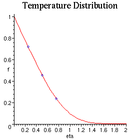
Evaluate Maple answer at specific points, compare to book answer on graph

> for i from 1 to 3 do fp[i]:=simplify(f(i*.25)) od;

> with(plots): with(plottools):

> p1:=point(plot(fbook(eta),eta=0...2)):

> p2:=point([.25,fp[1]],color=blue):

> p3:=point([.5,fp[2]],color=blue):

> p4:=point([.75,fp[3]],color=blue):

> plo:=[op(p1),p2,p3,p4]:

> display(plo,labels=["eta","f"],title="Temperature Distribution");