Introduction:

Example 11.1-2 explores the heating of a finite slab.  This problem is displayed in the notes to Ceng 402 and also in BS&L.  The answer is equation 11.1-31:

Here, this equation varies with respect to time and distance y.  First, we will explore the variation of Theta with respect to time at a constant value of y and then we will explore the variation of Theta with respect to y with a constant value of time.  Finally, we will combine the two and see a 3-dimensional plot of how Theta varies with respect to y and time.

For this problem, the thermal conductivity, density, and specific heat are all considered constant.  We have chosen the corresponding data to correlate with a slab of Iron shown with initial conditions below:

Theta vs. Time

In Theta vs. Time, we need to chose an arbitary distance y between the center of the slab and b, the outer edge.  Then we solve 11.1-31 for time, t:

> restart;
> untime:= s;

> g:= 60;amount of time in untime, for this case we've chosen 60 seconds

> k:= 30*Btu/s/3600/ft/F; the thermal conductivity

> rho:= 436*lbm/ft^3; the density

> Cp:= .12*Btu/lbm/F; the specific heat

> alpha:= k/rho/Cp; defining alpha

> y:= .01/12*ft; our arbitrary distance from the center

> b:= 1/12*ft; the distance from the center in our case

> alpha*t*untime/b^2; checking to make sure this term is free of units

> theta:= t-> 2*sum((-1)^n/((n+.5)*Pi)*exp(-(n+.5)^2*Pi^2*alpha*t*untime/b^2)*cos((n+.5)*Pi*y/b),n=0..50); equation 11.1-31 with time, t as the variable, we use only 50 iterations due to the limits of computing time and power instead of infinity.  This does not affect our results and is accurate enough.

> Theta:= [[t, theta(t)] $t=1..g]; running a small loop to calculate values to plot

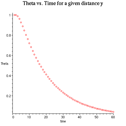
> plot(Theta, t = 0..g, style=point, symbol=circle, labels=["time","Theta"], title="Theta vs. Time for a given distance y");

Now we will solve for a specific temperature T at y = .01 ft. and time = 5 seconds given the fluid temperature at 270 degrees F and the initial slab temperature of 70 degrees F.
> T1:= 270*F;

> T0:= 70*F;

> eqn:= theta(5) = (T1-T)/(T1-T0); time is 5 seconds, notice theta here is a function of t

> solve(eqn, T);

Theta vs. Y

In Theta vs. y, we need to chose an arbitary time t and solve for y, the distance between the center of the slab and b, the outer edge.  Then we solve 11.1-31 for this distance, y.  This follows the plot on page 356 of BS&L where the lines drawn are for constant values of alpha*t/b^2 or different constant values of t.  Notice how theta here is (T1-T) / (T1-T0), the right axis.

> restart;

> unlength:= ft;

> h:= 60;  the number of divisions of b, incriments of y between 0 and b

> t:= 15*s; our arbitrary time, 15 seconds

> k:= 30*Btu/s/3600/ft/F;

> rho:= 436*lbm/ft^3;

> Cp:= .12*Btu/lbm/F;

> alpha:= k/rho/Cp;

> b:= 1/12*ft;

> theta:= y-> 2*sum((-1)^n/((n+.5)*Pi)*exp(-(n+.5)^2*Pi^2*alpha*t/b^2)*cos((n+.5)*Pi*y*unlength/b),n=0..50); equation 11.1-31 with distance, y as the variable, we use only 50 iterations due to the limits of computing time and power instead of infinity.  This does not affect our results and is accurate enough.
 

> Theta:= [[y*b/h/unlength, theta(y*b/h/unlength)] $y=1..h]: running a small loop to calculate values to plot

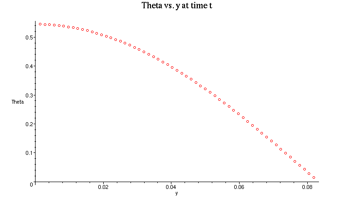
> plot(Theta, y = 0..1/12, style=point, symbol=circle, title="Theta vs. y at time t", labels=["y","Theta"]);

Now we will solve for a specific temperature T at t = 15 seconds and y = .04 ft. given the fluid temperature at 270 degrees F and the initial slab temperature of 70 degrees F.
> theta(.04);

> T1:= 270*F;

> T0:= 70*F;

> eqn:= theta(.04) = (T1-T)/(T1-T0);

> solve(eqn, T);

Theta vs. Y and t

Now that we've explored how theta varies with y and how theta veries with t, we can take it a step farther with the help of Maple and see how Theta varies with Y and t simultaneously.  This enhances the plot on page 356 by allowing us to also vary time in addition to y/b.  We use t and y instead of finding arbitrary values for t and y and then solve equation 11.1-31 for distance, y and time, t:

> restart;

> unlength:= ft;

> h:= 36; number of divisions of distance b

> untime:= s;

> g:= 60; time spread from zero to this number in units the time

> k:= 30*Btu/s/3600/ft/F;

> rho:= 436*lbm/ft^3;

> Cp:= .12*Btu/lbm/F;

> alpha:= k/rho/Cp;

> b:= 1/12*ft;

> alpha*t*untime/b^2;

> theta:= (t,y)-> 2*sum((-1)^n/((n+.5)*Pi)*exp(-(n+.5)^2*Pi^2*alpha*t*untime/b^2)*cos((n+.5)*Pi*y*unlength/b),n=0..25); equation 11.1-31 with time, t and distance, y as the variables, we use only 25 iterations due to the limits of computing time and power instead of infinity.  This does not affect our results and is accurate enough and still takes a decent amount of time.

> Theta:= array(1..g,1..h); establishing arrays to calculate Theta(t,y)

> for u from 1 to g by 1 do
for z from 1 to h by 1 do Theta[u,z]:= (theta(u,z*b/h/unlength)) od od: This double for loop calculates the t and y values for each corresponding position in the array Theta[t,y] first calculating the time from 1 to g and then the distance from 1 to h as specified above.

With this array, we can create a 3-dimentional plot that shows Theta as a function of y and time over the distance 0 = y = b ft. and the time 0 = t = 60 seconds:
> plot3d(Theta[x,y], x = 1..g,y=1..h, axes=boxed, labels=["time","h (=y/b from 0 to 1)", "Theta"], title="Theta as a function of y and time");

The plot is logical with the upper corner showing where time equals zero and the distance y = zero so that the initial Theta = 1 or T = T1.  Correspondingly, the plot also displays at time = 60 seconds and distance y = b, Theta equals 0 or nearly 0 indicating that T = To.  With this array of Theta values, you could calculate for T using any time between 0 and 60 seconds and any y value between 0 and 1/12 of a foot.