Example 10.6-2:

Surface Temperature of an Electric Heating Coil

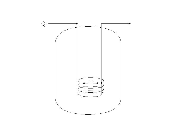
PROBLEM STATEMENT: An electric heating coil of diameter D is being designed to keep a large tank of liquid above its freezing point. It is desired to predict the temperature that will be reached by the coil surface as a function of the heating rate Q and the tank surface temperature T0. This prediction is to be made on the basis of experiments with a smaller geometrically similar apparatus filled with the same liquid. Outline a suitable experimental procedure for making the desired prediction. Temperature dependence of the physical properties other then rho may be neglected, and the entire heating coil surface may be assumed to be at the same temperature, T1.

SOLUTION:

restart;

The following is equation 10.6-19 from the book. The integral is perfromed over the surface area of the coil, A, at the conditions of the fluid immediately adjacent to the soils surface.

> Q:=-k*Int(diff(T(r),r),A);

To rewrite the equation in terms of dimensionless variables, we must first define the dimensionless parameters, and then substitute them into the equation using the PDEtools.

> tr:={T(r)=T0+Tstar*(T1-T0), r=D*rstar, A=Astar*D^2};

> with(PDEtools, dchange);

The following is now 10.6-20 from the book, with a little algebra. the (T1-T0) and D terms and constant and can be pulled out of the integral. Then, we can divide the equation by D, k, and (T1-T0) to get the equation exactly as it appears in the book.

> Q:=dchange(tr,Q,[rstar, Astar, Tstar(rstar)]);

equation 10.6-19 can also be expressed in terms psi, a funtion of the Prandtl and Grashof numbers. First the Grashof and Prandtl numbers must be defined,

> Pr:=Cp*mu/k; Gr:=rho^2*beta*(T1-T0)*g*D^3/mu^2;

and the equation becomes:

> unassign('Q'); DimEq:=Q/k/D/(T1-T0)=psi(Pr,Gr);

Multiplying both sides of the equation yields equation 10.6-26:

> DimEq:=DimEq*Gr;

We may solve this equation for (T1-T0). The Prandtl number can be considered constant because we are neglecting the temperature dependence of the physical properties. The coefficient of the RHS of the above equation is simply the grashof number and can be included in the function psi. Doing so, solving the equation for (T1-T0), and defining the function phi of the LHS of the above equation (to be determined experimentally) simplifies the expression to :

> DimEq:=(T1-T0)=(T1-T0)/Gr*phi(lhs(DimEq));

This equation can be plotted using experimental values for T1, T0, D, and the physical properties of the fluid. This plot could then be used to predict the behavior of the larger system. If the ratio Q in the two systems is maintained as inversly proportional to the square of D, then the ratio (T1-T0) will be inversely proportional to D^3.