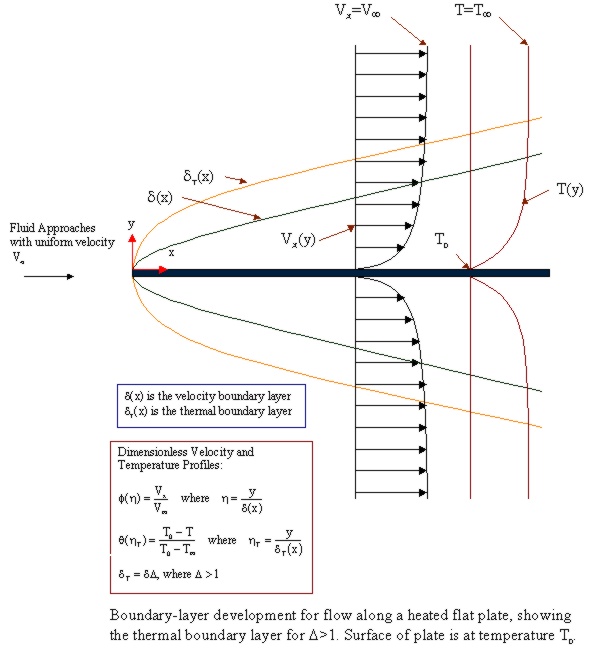
The temperature profile as a fluid passes around a solid is often flat except in regions near the solid surface.  Boundary layer theory is applied to obtain a solution for the region near a flat plate
where heat transfer is assumed to be in the steady state.   The wet surface of the plate has a constant temperature of T0 and the fluid approaching the plate from the left has temperature T_infinity.  In this problem, the momentum boundary layer is within the thermal boundary layer.  An illustration of the momentum and thermal boundary layers surrounding the flat plate is shown in the
diagram below.
 
 

NOTE: The italicized points highlight how the method of solution of this problem differs from the method of solution of Example 11.4-1.

I. Define the two differential equations that describe the fluid flow near the flat plate. These are the steady-state equation of continuity and the x-component of the equation of motion. The y-component of the equaton of motion is not considered because there is little flow in the y-direction.

II. Solve the equation of continuity for vy. Enter the assumed form for vx as defined by Eqs. 11.4-4,5. Substitute vx and vy into the x-component of the equation of motion.

III. The x-component of the equation of motion is in terms of x and y. In a first step towards eliminating y, the equation of motion is integrated from y=0 to y = delta(x). This will result in equation equivalent to Eq. 4.4-19 (from chapter 4).

IV. Define the equation of energy. Since the thermal boundary layer is outside of the momentum boundary layer, the equation of energy will be divided into two regions, one inside the momentum boundary layer and one outside the momentum boundary layer.The velocity of the fluid in the y-direction outside of the momentum boundary layer will have the same velocity as it had at the momentum boundary layer.

> eengin:=(x,y)->vx(x,y)*D[1](T)(x,y)+vy(x,y)*D[2](T)(x,y)-alpha*D[2](D[2](T))(x,y);

> eengout:= (x,y)->vinf*D[1](T)(x,y)+vy(x,delta(x))*D[2](T)(x,y)-alpha*D[2](D[2](T))(x,y);

V. Enter the assumed form of the temperature profile.

VI. The region within and outside of the momentum boundary layer each have a separate energy equation. In a first step towards eliminating y in these equations, the inner equation is integrated from y=0 to y=delta(x) and the outer equation is integreated from y=delta(x) to y=delta(x)*Delta where Delta is the ratio of the thickness of the thermal boundary layer to the thickness of the momentum boundary layer. The two integrals are added to get an equation 11 analagous to the equation 11 found in the case where the momentum boundary layer was outside of the thermal boundary layer.

> eq11in:=int(eengin(x,y),y=0...delta(x)); Eq. 11 on page 368

> eq11out:=int(eengout(x,y),y=delta(x)...Delta*delta(x));

> eq11:= eq11in+eq11out;

VII. To eliminate y from the previous equations, a velocity profile and a temperature profile must be selected. The velocity profile must be zero at eta = 0 and have a zero derivative at eta=1. The temperature profile must be zero at etaT = 0, one at etaT = 1, and have zero first and second derivatives at etaT=1.

VIII. Recall equation 11 followed from the equation of motion and equation 19 followed from the equation of motion. Now the velocity and temperature profiles will be substituted into the equations and the left-hand side of each equation will be set to zero.

IX. Since equation 19 involves only delta(x), it is solved for delta(x) by using the boundary condition delta(x) = 0 at x = 0. Choose the solution that gives positve delta(x).

X. Now that an equation for delta(x) exists, it can be substituted into equation 11 to yield an equation involving Delta.

XI. Substitute in the equation relating alpha to Prandtl number and solve for the Prandtl number. The resulting equation relates Delta to the Prandtl number. You can now show that your solution is equivalent to the desired answer.