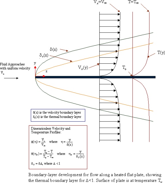
The temperature profile as a fluid passes around a solid is often flat except in regions near the solid surface.   Boundary layer theory is applied to obtain a solution for the region near a flat plate where heat transfer is assumed to be in the steady state.   The wet surface of the plate has a constant temperature of T₀ and the fluid approching the plate from the left has temperature T_infinity.  In this problem, the thermal boundary layer is within the momentum boundary layer.  A separate problem could be considered where the thermal boundary layer is outside the velocity boundary layer.   An illustration of the velocity and thermal boundary layers surrounding the flat plate are shown in the diagram below.
 
 

> restart;

First, we will start with equations that determine the fluid flow. Later, we will define the equation of energy of the fluid and use these equations together to relate the Prandtl number to Delta, the ratio of the thermal boundary layer thickness to the velocity boundary layer thickness.

Define the two differential equations that describe the fluid flow near the flat plate. These are the steady-state equation of continuity and the x-component of the equation of motion. The y-component of the equaton of motion is not considered because there is little flow in the y-direction.

Continuity equation (Eq. 11.4-1)

Note: D[1] represents derivative with respect to x and D[2] represents derivative with respect to y

> eq_cont:=D[1](vx)(x,y)+D[2](vy)(x,y)=0;

x-component of equation of motion (Eq. 11.4-2)

Note: The D[2](D[2](vx))(x,y) is neglected because it is small compared to the vx(x,y)*D[1](vx)(x,y) term. Also, eq_motx in its present form is not an equation. In solving for Delta, the final differential equation will be set equal to zero.

> eq_motx:=(x,y)->vx(x,y)*D[1](vx)(x,y)+vy(x,y)*D[2](vx)(x,y)-nu*D[2](D[2](vx))(x,y);

Solve the equation of continuity for vy. Enter the assumed form for vx as defined by Eqs. 11.4-4,5. profile equation. Substitute vx and vy into the x-component of the equation of motion.

Solve for vy using the boundary condition that vy = 0 at y = 0.

> vy:=(x,y)->-int(D[1](vx)(x,y1),y1=0...y);

Assumed form for vx(x,y)

> vx:=(x,y)->vinf*phi(y/delta(x));

Substituting vy into the x-component of the equation of motion yields the following equation

> eq_motx(x,y);

The x-component of the equation of motion is in terms of x and y. In a first step towards eliminating y, the equation of motion is integrated from y=0 to y = delta(x). This will result in equation equivalent to Eq. 4.4-19 (from chapter 4).

> eq_19:=int(eq_motx(x,y),y=0...delta(x));

The equation of energy will now be defined.

Equation of energy (Eq. 11.4-3)
Note: eq_engy in its present form is not an equation. In solving for delta(x), the final differential equation will be set equal to zero.

> eq_engy:=(x,y)->vx(x,y)*D[1](T)(x,y)+vy(x,y)*D[2](T)(x,y)-alpha*D[2](D[2](T))(x,y);

Enter the assumed form of the temperature profile in the thermal boundary layer as shown in Eqs. 11.4-6,7.

> T:=(x,y)->T0+(Tinf-T0)*Theta(y/(Delta*delta(x)));

The equation of energy in its present form contains both x and y. In a first step towards eliminating y, the equation of energy is integrated from y=0 to y=delta(x)*Delta where Delta is the ratio of the thickness of the thermal boundary layer to the thickness of the velocity boundary layer. In this problem, Delta is less than 1 because the thermal boundary layer is within the velocity boundary layer.

Eq. 11.4-11

> eq_11:=int(eq_engy(x,y),y=0...Delta*delta(x));

To eliminate y from the previous equations, a velocity profile and a temperature profile must be selected. The velocity profile must be zero at eta = 0 and have a zero derivative at eta=1. The temperature profile must be zero at etaT = 0, one at etaT = 1, and have zero first and second derivatives at etaT=1. Many profiles could be used. The ones selected by Bird, Stewart, and Lightfoot are used below.

Velocity profile (Eq. 11.4-17)

> phi:=eta-> 2*eta-2*eta^3+eta^4;

Temperature profile (Eq. 11.4-18)

> Theta:=etaT->2*etaT-2*etaT^3+etaT^4;

Recall eq_19 followed from the equation of motion and eq_11 followed from the equation of energy. Now the velocity and temperature profiles will be substituted into the equations and the left-hand side of each equation will be set to zero.

eq_11 is a 1st order equation in delta(x), but Delta is present also. At this stage, set the left hand side of eq_11 equal to zero.

> eq_11:=simplify(eq_11/(Tinf-T0))=0;

This is a 1st order ODE that involves only delta(x). At this stage, set the left hand side of eq_19 equal to zero.

> eq_19=0;

Since eq_19 involves only delta(x), it is solved for delta(x) by using the boundary condition delta(x) = 0 at x = 0.

Note: Two solutions exist. Choose the solution which gives positive delta(x)

> s:= dsolve({eq_19, delta(0)=0}, delta(x));

Choose the function that gives positve delta(x)

> assign(s[2]); delta:= unapply(delta(x),x);

Now that an equation for delta(x) exist, it can be substituted into eq_11 to yield an equation for Delta

> eq_11;

Substitute in equation for alpha as a function of Prandtl number and solve for the Prandtl number.

> alpha:= nu/Pr;

> Pr:= solve(eq_11,Pr);

Show that this equation relating the Prandtl number and Delta is equivalent to equation 11.4-20 in the textbook.

> simplify(37/(630*Pr)-Delta^3/15+3*Delta^5/280-Delta^6/360);

The solution presented is correct and is valid for the assumed velocity and temperature profiles shown in equations 11.4-17 and 11.4-18.