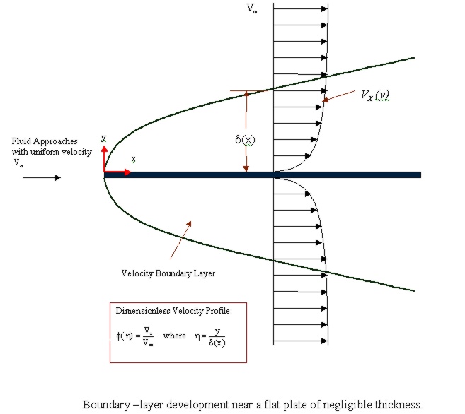
Ideal flow solutions do not yield accurate description of fluid flow near a plate because of the no-slip condition which occurs at the plate surface.  Consequently, boundary layer theory must be used to describe fluid flow near the plate surface.  Boundary layer theory is used to find an approximate description of fluid flow, taking viscous drag into account, in a thin boundary region near the plate.  In this problem, the momentum boundary layer thickness, delta, as a function of position will be determined.   No thermal boundary layer exists because the fluid and the plate are isothermal.

> restart;

First, define the two differential equations that describe the fluid flow near the flat plate. These are the steady-state equation of continuity and the x-component of the equation of motion. The y-component of the equaton of motion is not considered because there is little flow in the y-direction .

Continuity equation (Eq. 4.4-12)

Note: D[1] represents derivative with respect to x and D[2] represents derivative with respect to y

> eq_cont:=D[1](vx)(x,y)+D[2](vy)(x,y)=0;

x-component of equation of motion (Eq. 4.4-13)

Note: The D[2](D[2](vx))(x,y) is neglected because it is small compared to the vx(x,y)*D[1](vx)(x,y) term. Also, eq_motx in its present f orm is not an equation.

Before solving for delta(x), the resulting differential equation will be set equal to zero.

> eq_motx:=(x,y)->vx(x,y)*D[1](vx)(x,y)+vy(x,y)*D[2](vx)(x,y)-nu*D[2](D[2](vx))(x,y);

Solve the equation of continuity for vy and and substitute vy into the x-component of equation of motion.

Solve for vy using the boundary condition that vy = 0 at y = 0.

> vy:=(x,y)->-int(D[1](vx)(x,y1),y1=0...y);

Substituting vy into the x-component of the equation of motion yields Eq. 4.4-14.

> eq_motx(x,y);

The x-component of the equation of motion will be used to solve for vx. This nonlinear equation will be solved with the following boundary conditions:

vx = 0 at y=0,

vx = vinfinity at y = infinity,

vx = vinfinity at x = 0 for all y

As an approximation, assume the velocity profiles at different values of x have the same shape. The assumed form of the velocity profile is entered below.

Assumed form of solution (Eq. 4.4-15)

> assume(vinfinity>0);

> vx:=(x,y)->vinfinity*phi(y/delta(x));

The x-component of the equation of motion is shown below after substitution of assumed form of vx

> eq_motx(x,y);

The x-component of the equation of motion is presently in terms of x and y. In a first step towared eliminating y, the equation of motion is integrated from y=0 to y = delta(x). This will result in equation equivalent to Eq. 4.4-19 .

> eq_19:=int(eq_motx(x,y),y=0...delta(x));

To eliminate y, a velocity profile phi which is function of eta must be selected. The profile must be zero at eta = 0 and have a zero derivative at eta=1. Many profiles could be used. The one selected by Bird, Stewart, and Lightfoot is used below .

phi:=eta->(3/2)*eta-(1/2)*eta^3;

The simplified differential equation that determine the thickness of delta at postion x. At this time, the left hand side of equation 19 will be set to zero.

> eq_19=0;

The differential equation obtained can now be solved for delta(x) using the boundary condition that delta(x) = 0 at x = 0

Solve for delta(x)

Note: Two solutions will be obtained.

> s:=dsolve({eq_19,delta(0)=0},delta(x));

Choose solution that gives positive delta.

> assign(s[2]);

Evaluate delta(x) to get a numerical value for its coefficient.

> delta(x):=simplify(evalf(delta(x)));

The delta(x) obtained is the same as the solution presented in Bird, Stewart, and Lightfoot (Eq. 4.4-25) for the velocity profile phi(eta)=(3/2)*eta-(1/2)*eta^3 .