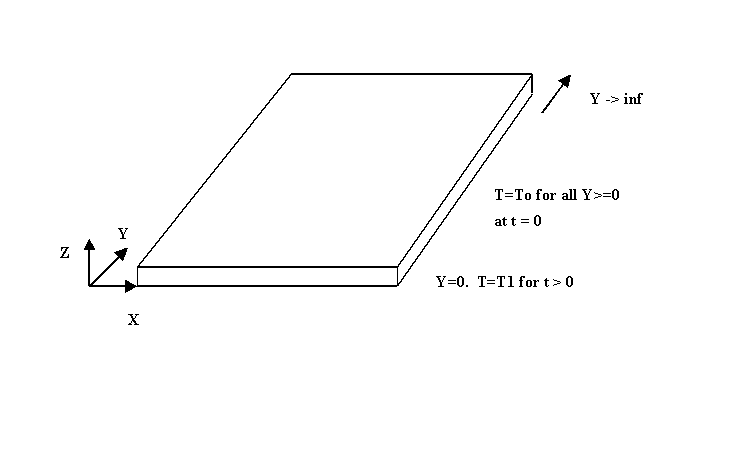
Example 11.1-1 Heating of a Semi-infinite Slab

Whitney Smith and Andy Edgar

Ceng 402 Project, April 28, 2000.

A solid body occupying the space from y=0 to y=inf is initially at temperature To. At time t=0, the surface at y=0 is suddenly changed to temperature T1 and maintained at the temperature for t > 0. Find the time dependent temperature profiles T(y,t).

> restart;

eq. 11.1-3 - Equation 11.1-2 modified for dimensionless temperature profile Theta = (T-To)/(T1-To) and with respect to y. Alpha = k / (rho*Cp), the thermal diffusivity of the solid. k is the thermal conductivity, rho the density, and Cp the heat capacity at constant pressure.

> eq:=D(Theta)(t)=alpha*D(D(Theta))(y);

Define eta as in chapter 4 (ex. 4.1-1), dimensionles variable in terms of y.

> eta:=y/sqrt(4*alpha*t);

Use the chain rule on left hand side of eq

> chain1:=D(Theta)(eta)*diff(eta,t);

Chapter 11 equivalent of right hand side of equation 4.1-5. (Phi = Theta)

> bookeq1:=D(Theta)(eta)*(-.5)*eta/t;

Prove book equation is the chain rule expansion of D(Theta)(t), ie. that equation 4.1-5 is true for this example.

> simplify(chain1-bookeq1);

Use chain rule to expand right hand side of eq.

> chain2:=D(D(Theta))(eta)*diff(eta,y)*diff(eta,y);

Chapter 11 equivalent of right hand side of equation 4.1-6.

> bookeq2:=D(D(Theta))(eta)*eta^2/y^2;

Prove book equation is the chain rule expansion of D(Theta)(t), ie. that equation 4.1-6 is true for this example.

> simplify(chain2-bookeq2);

Rearranging eq in terms of the chain rule expansions defined above.

> bigeq:=alpha*chain2-chain1=0;

> simplify(bigeq);

Further simplification shows that 1/(4*t) is common to both terms and can be eliminated from the equation.

> eq3:=simplify(4*t*bigeq);

Return eta to its variable form to leave solution in dimensionless form.

> eta:='eta';

To get back to dimensionless form, define y in terms of eta.

> y:=2*eta*sqrt(alpha*t);

Dimensionless form of eq

> eq4:=simplify(eq3);

Solve eq using dsolve and boundary conditions given in equations 11.1-5 and 11.1-6.

> s:=dsolve({eq4,Theta(0)=1,Theta(inf)=0},Theta(eta));

> assign(s); Theta:=unapply(Theta(eta),eta);

To simplify, we see that as n goes to infinity, erf(n) goes to 1.

> evalf(erf(1000000));

In light of this, define erf(inf) as 1.

> erf(inf):=1;

Simplify solution to get equation 11.1-7.

> Theta(eta):=simplify(Theta(eta));

Since eta depends on both y and t, this solution is the dimensionless temperature profile in terms of both variables.

Now for a numerical example.

We begin with the equation developed above for Theta.

> restart;

> eq:=Theta=1-erf(eta);

State the definitions of the dimensionless parameters Theta and eta.

> Theta:=(T-To)/(T1-To); eta:=y/sqrt(4*alpha*t);

Show that the definition of the Theta equals the solution we developed for Theta.

> eq;

Solve the equation originally in terms of Theta for T.

> T:=solve(eq,T);

Define given constants for the case where the slab is made of steel (constants from BS&L Problem 11D).

> k:=25*4.1365e-3*cal/s/cm/C; rho:=7.7*g/cm^3; Cp:=.12*cal/g/C;

> To:=(1000-32)*5/9*C; T1:=(200-32)*5/9*C;

> alpha:=k/rho/Cp;

Use the equation solved for T above to find the temperature at a given height y in the slab at a time t after the surface temperature is changed.

> y:=1*cm; t:=10*s; simplify(T,assume=positive);

> y:=100*cm; t:=1000*s; simplify(T,assume=positive);

> y:=1*cm; t:=1000*s; simplify(T, assume=positive);

>