Example Problem 19.1-2 in BS&L

Solution by James Bradley Aimone

CENG 402 – April 2000

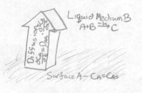Interpretation of Problem –

Substance A is diffusing

from a surface up into a

liquid medium B. Once in

this medium, A begins to

react with B to form a third product – C. To model

the concentration of A, the basic law of diffusion is

applied and a loss term due to the reaction is taken

as well.

BS&L proposes a solution to the problem which is to be

tested here. The first method shown took the proposed

solution and plugged it into the original equation,

and the second method had Maple solve the equation and

compared Maple’s solution to BS&L’s.

> restart;with(PDEtools); Restarts and activates Partial Differential Eqn. functions

> Diffgain:=Dab*diff(Ca(x,t),x,x);Rxnloss:=-k*Ca(x,t); Amount gained by diffusion into system, and amount lost by conversion from A->B

> In:=Diffgain:Out:=Rxnloss:

> Acc:=In-Out;consv:=Acc=diff(Ca(x,t),t): Balanced equation of conservation of mass - equal to eq. 19.1-23

>

> sltn:=pdsolve(Acc=diff(Ca(x,t),t),build); Maple's solution of equation 19.1-23

> sltneq:=Ca(x,t)=C*exp(t*Dab*a)*exp(t*k)*A*sinh(a^.5*x)+C*exp(t*Dab*a)*exp(t*k)*B*cosh(a^.5*x); Allows us to test the solution Maple gives us

> pdetest(sltneq,consv); A test of Maple's solution If 0, then it is correct

Yep, Maple's solution is correct...of course.

> sltneq:=(x,t)->C*exp(t*Dab*a)*exp(t*k)*A*sinh(a^.5*x)+C*exp(t*Dab*a)*exp(t*k)*B*cosh(a^.5*x); Making Maple's solution a function we can work with

> sltneq(x,0);

Note - if the solution sltneq=0 when t=0, then either C=0 or A=B=0, either of which would make the problem trivial.

therefore the boundary conditions will not be applied at this moment.

Anyway, the above solution is Maple's solution to the differential equation that was introduced.

Now the test of BS&L's solution

> pdsolve(diff(Ca(x,t),t)=Dab*diff(Ca(x,t),x,x),build); Solving eq. 19.1-23 for k=0

> f:=(x,t)->C*exp(Dab*a*t)*A*sinh(a^.5*x)+C*exp(Dab*a*t)*B*cosh(a^.5*x); f(x,t) is obtained from the equality Dab*d2f/dx2=df/dt

> BSLsln:=(x,t)->-k*(int(f(x,t1)*exp(k*t1),t1=0...t))+f(x,t)*exp(k*t); From eq 19.1-26, which BS&L claim is the solution

> consv;

> Ca(x,t):=BSLsln(x,t);

> consv;

> simplify(consv); Reduced equality shows that the equation is not entirely equal - that there is a leftover set of terms

> solve(consv,A); An equality in the leftover set of terms allows a value for A to be found - which shows this calculation is wrong

First method of plugging in BS&L into original equation did not work… Now for the second method –

> BSLsln(x,t);BSL0t:=BSLsln(x,0):BSL0x:=BSLsln(0,t):

> testeqn:=BSLsln(x,t)=sltneq(x,t); Second test is to try to equate BS&L's solution to the one Maple gave us earlier.

> t1:=simplify(testeqn/C*(Dab*a+k)); This solution to the equality is similar but not exactly equal to the result from previous test.

> solve(t1,A); Maple cannot determine a value for A, showing that no equality is found in t1. Therefore, the solution can be considered complete.

> h:=BSL0t=sltneq(x,0); When t=0, the equality can be seen easily

Proof that BS&L solutions abide by the boundary conditions....

Since it is known that f=Cas on the surface, we'll test the original BS&L solution for this quality-

> Casu:=-k*int(fs(x,t2)*exp(k*t2),t2=0...t)+fs(x,t)*exp(k*t); fs(x,t):=Casur;fs(x,t2):=Casur;Casu;

> simplify(Casu); Simplifying the answer shows us that the concentration at the surface is really independent of time. Therefore the BS&L solution matches this boundary condition as well.

> Cat:=-k*int(ft(x,t2)*exp(k*t2),t2=0...t)+ft(x,t)*exp(k*t); ft(x,t2):=0: ft(x,t):=0: Cat;

It is shown here that the BS&L solution for 19.1-23 abides by the initial condition of Ca=0.

The second method of equating the Maple solution to the BS&L solution worked, and when the BS&L solution was tested for boundary conditions it passed.