Calculation of Heat-Transfer Coefficients from Experimental Data
Section 13.1; Bird, Stewart and Lightfoot

---

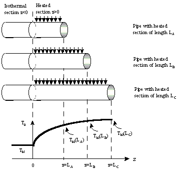
This example involves calculating heat transfer coefficients from experimental data by heating air in tubes of various lengths. Air is flowing with fully developed laminar velocity profiles in each tube at a temperature of 200 F. At z=0, the temperature of each pipe is suddenly increased to 212 F. The air temperature at the exit of each tube is measured. The following picture is a representation of Fig. 13.1-2.




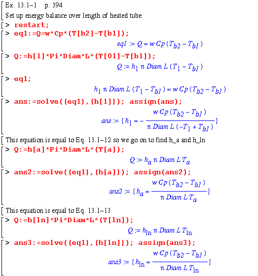
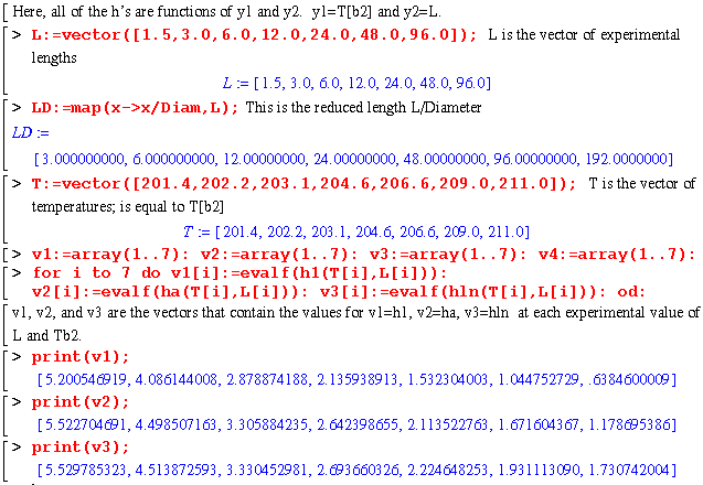
By setting up an energy balance and equating wuth equations 13.1-(2-4), h1, ha, and hln can be solved for symbolically.





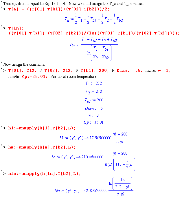
Now the experimental data is plugged into the equations for the heat transfer coefficients defined above.



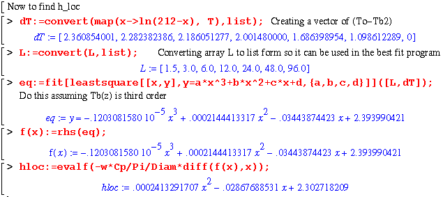
H_loc is a bit more difficult to find and will vary in precision because it involves a differential.



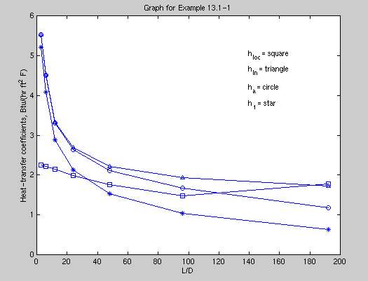
Plugging the vectors for all of the h's into Matlab gives the following graph. This graph matches precisely for the values of h1, ha, and hln. Hloc is calculated from the slope of the best fit curve of ln(To-Tb) vs. L from Maple and evaluated in Eq. 13.1-18. Hloc varies somewhat, but approaches its minimum value at the same asymptote that hln is approaching. You can see that hloc approaches the asymptote more rapidly than hln though.

---