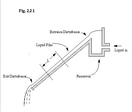
First, we will look at Figs. 2.2-1 and 2. Fig. 2.2-1 illustrates the end effects of the falling film.

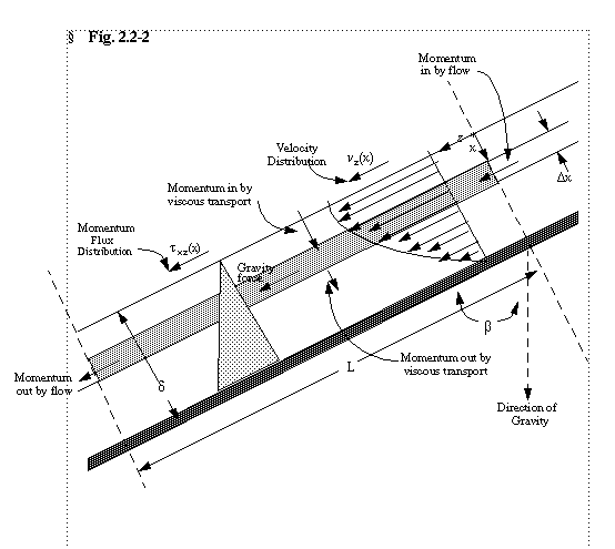
Fig. 2.2-2 illustrates the flow of the viscous liquid film under gravitational influence with no rippling. The energy balance is made over a slice of thickness delta(x). In this diagram, the y-axis points outward from the screen.
We will start by going back to chapter 2 in BS&L to look at the derivation of the equations that govern flow in a film on an inclined plane surface.
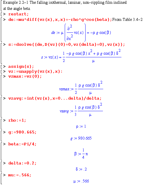
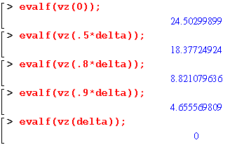
The properties are expressed in cgs units for water over the range of temperatures: 0 to 100C. The viscosity was determined at the average temoerature: 50C. Here are the velocities at various points in the film in cm/s.
Here is the first case where variable viscosity is treated. Its dependence on position in the film is assumed to be exponential as specified by eq. 2.2-22. The stress can be found just as for the first case, but the equation that determines the velocity is more complex.
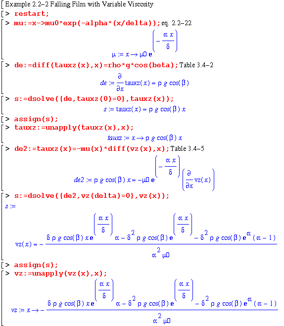
Let's see if that function agrees with equation 2.2-24.
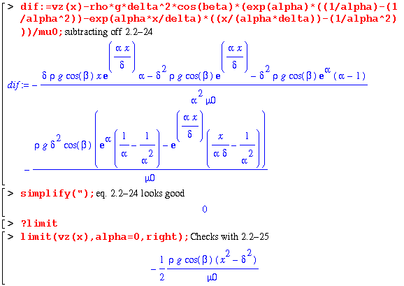
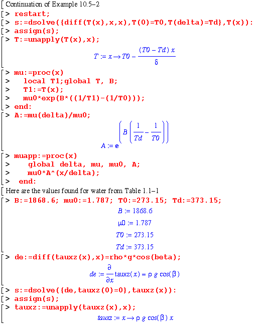
It does check and it has the right limit as the parameter alpha goes to 0. Now we can go on to Example 10.5-2. The temperature is a simple linear function of distance in the film. Some problems were encountered in trying to define a function of a function to get the dependence of mu on distance so a procedure was used to do this.
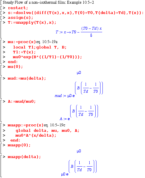
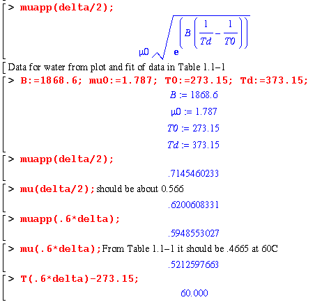
The approximation used for mu as a function of distance was needed so the equation for velocity in a film with varying viscosity from section 2.2 in Example 2.2-2 could be used. We compared the approximations for mu for water over the temperature range 0 to 100C. The function muapp gave much larger errors in viscosity than the mu function.
|
|
|
|
|
|
|
|
|
|
|
|
|
|
|
|
|
|
|
|
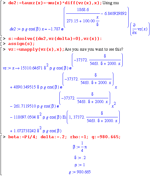
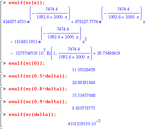
Those velocities were found using the better mu approximation: eq. 10.5-19a. Now we will compare it with the approximation 10.5-19c (or 10.5-19.)
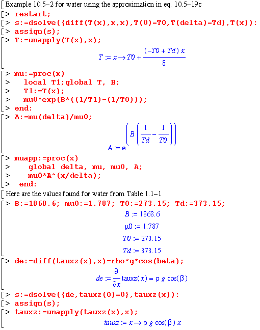
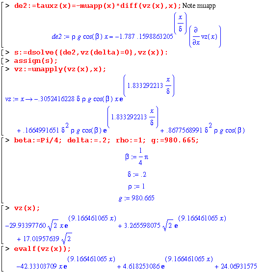
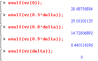
Certainly both approximations are much better than the use of the average temperature to determine mu and then use the isothermal assumption.
|
|
|
|
|
|
|
|
Isothermal using mu at average temperature |
|
|
|
|
|
|
Nonisothermal using approximation in 10.5-19 |
|
|
|
|
|
|
Nonisothermal using fit of data with eq. 10.5-19a |
|
|
|
|
|