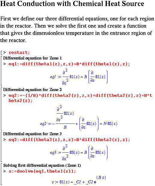
First we define our differential equations: three of them, one for each region in the reactor. Then we solve the first one and create a function that gives the dimensionless temperature in the entrance region of the reactor.

That solves the second equation for the region where the reaction is taking place, but we need to make it into a function as well. We will treat the third region at the end of this secion and look at all three functions. In the entrance and exit parts we have also used the boundary conditions at plus and minus infinity.
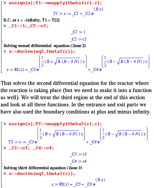
Now we need to choose the remaining four parameters to satisfy the other four boundary conditions.
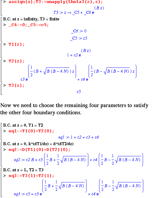
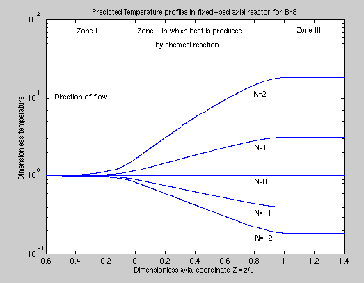
This is really going to be long! We can try to get a numerical solution that should match one of the curves in Figure 9.5-2.
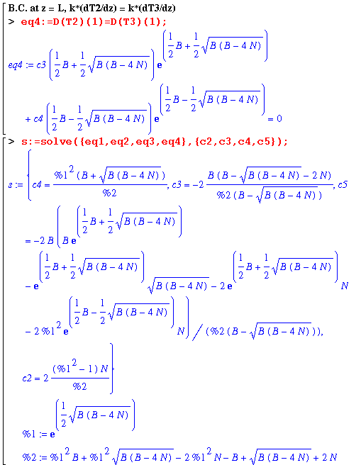
That doesn't look too good, but if we examine the solution, we find that those parameters lead to a solution in which there is a double root and it is not surprising that we got an error. If we try another value for N, things look a lot better. We can also create a single function that will give the temperatures at all parts of the reactor.
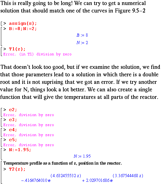
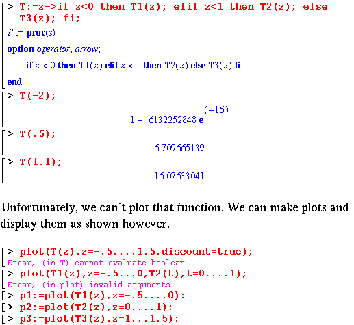
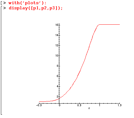
Unfortunately, we can't plot that function. We can make plots and display them as shown however.
