The Cooling fin which requires the least material

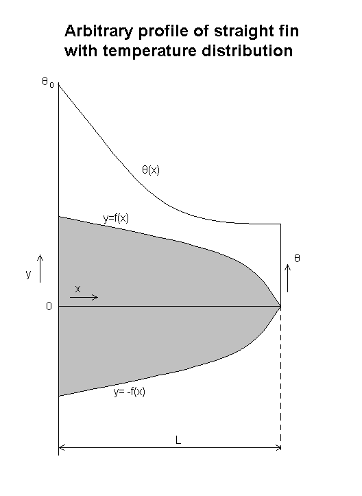
Here we will derive the general equation for heat flux for a fin given an arbitrary profile.  Since the Width of a colling fin is often dictated by what it is we are trying to cool, we will ignore that dimension and only concentrate on the dimensions of the profile. The length and the equation generating the profile.  For example the fin could be a rectangular one, a triangular one, or any shape for that matter.  Here we will calculate the optimal fin profile.  This profile will minimize the material needed for a given total heat loss.

> restart;

The heat flux at a point is given by this equation, the standard Newton's Law of Cooling.

> q:=(y,x)->-k*y(x)*diff(theta(x),x);

The equation for heat loss from the surface.  Combined these two generate a formula that is dependant on the profile equation.
Note the dy/dx.  These are determined by the choice of a profile equation for the fin.

> eqn1:=-diff(q(y,x),x)=h*theta(x):
eqn2:=simplify(eqn1/k);

Find the total heat loss over the fin.

> eqn3:=qtot=h*int(theta(x),x=0...L);

The area of the profile, which is our value to be minimized.

> eqn4:=Area=int(y(x), x=0....L);

Now we would like to create a fin that uses the least material to give off the heat.
What f(x) minimizes this Area?

It would make sense that a linear equation for the temperature distribution would be the most efficient way to give off heat from the rod.  So we will try to find the profile equation that will give this type of linear temperature distribution.

Our linear equation for temperature "excess"

> theta:=x->theta0-m*x;

We can sub this back into our first equation and solve for a profile equation.

> ans:=dsolve({eqn2, y(L)=0},y(x)):
assign(ans):

> y:=unapply(y(x),x);

> eqn3;

> eqn4:=simplify(eqn4);

The slope must be this to satisfy our end conditions.  The excess is Theta0 for x=0, and 0 for x=L.

> m:=theta0/L;

Now we generate three important values here, the characteristic length, height, and area of the profile.  With these equations we can find the Length,Height, and resulting profile area that is necessary given:

•  a total heat to be removed

• an initial temperature of the rod

• surface heat transfer coefficient

• internal heat transfer coefficient.

These four values will determine the size of the fin necessary.  It is also important to note that these equations will seem remarkably similar as we progress on to fins of differing sizes.  This will allow us to compare different fins.

> L:=simplify(solve(eqn3,L));

> eqn4;
assign(eqn4):

> simplify(y(x));

Maple refuses to reduce this down, so we'll show it's equivalence to that formula found in the book.

> booky:=x->h/2/k*(x-2*qtot/h/theta0)^2;

> difference:=simplify(y(x)-booky(x));

Our three values, note that n is the ratio of the temperature excess at L to the temperature excess at zero.

> L_eqn:=L;
y0_eqn:=booky(0);
Area_eqn:=Area;
n:=theta(L)/theta0;

The resulting equation for the temperature distribution along the rod, linear as we expected, 
and the resulting profile equation which we can see is a quadratic.

> theta(x);
y(x);

> theta0:=1;
h:=1;
k:=1;
qtot:=1;

> with(plots):
p1:=plot(theta(x),x=0..L):
p2:=plot(y(x),x=0..L):
p3:=plot(-y(x),x=0..L):
display([p1,p2,p3]);

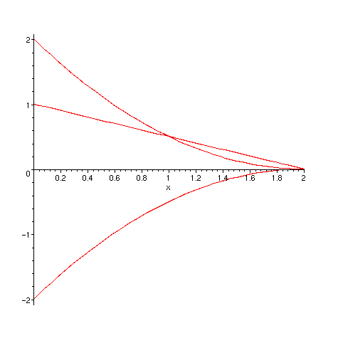
Here we have plotted the equations.  The linear one is the temperature profile, mostly as a quick visual aid to see that it is indeed linear.
The two curved lines show the profile of our fin.  Needless to say, although this may be a fin of minimum material, its sharp point at the end makes it hard to manufacture, and thus less useful.  This acute tip is impractical, so we will move on to one of the easier fins to manufacture, that of a rectangular fin.